Model-Independent Discrete Barrier Adjustments

I continue the investigation of discrete barrier approximations started in an earlier post. The idea is to find good approximations to a continuous barrier condition, while only sampling the process at a discrete set of times. The difference now is that I will look at model independent methods which do not explicitly depend on properties of the underlying process, such as the volatility. This will enable much more generic adjustments which can be applied more easily and more widely. I point out now, the techniques that I will describe here are original research and cannot currently be found in the literature outside of this blog, to the best of my knowledge.

Recall that the problem is to compute the expected value of a function of a stochastic process X,

(1)

which depends on whether or not the process crosses a continuous barrier level K. In many applications, such as with Monte Carlo simulation, we typically only sample X at a discrete set of times 0 < t₁ < t₂ < ⋯< t_n = T. In that case, the continuous barrier is necessarily approximated by a discrete one

(2)

As we saw, this converges slowly as the number n of sampling times increases, with the error between this and the limiting continuous barrier (1) only going to zero at rate 1/√n.

A barrier adjustment as described in the earlier post is able to improve this convergence rate. If X is a Brownian motion with constant drift μ and positive volatility σ, then the discrete barrier level K is shifted down by an amount βσ√δt where β ≈ 0.5826 is a constant and δt = T/n is the sampling width. We are assuming, for now, that the sampling times are equally spaced. As was seen, using the shifted barrier level in (2) improves the rate of convergence. Although we did not theoretically derive the new convergence rate, numerical experiment suggests that it is close to 1/n.

Another way to express this is to shift the values of X up,

(3)

Then, (2) is replaced to use these shifted values, which are a proxy for the maximum value of X across each of the intervals (t_i-1, t_i),

(4)

As it is equivalent to shifting the level K down, we still obtain the improved rate of convergence.

This idea is especially useful because of its generality. For non-equally spaced sampling times, the adjustment (3) can still be applied. Now, we just set δt = t_i – t_i-1 to be the spacing for the specific time, so depends on index i. It can also be used for much more general expressions than (1). Any function of X which depends on whether or not it crosses a continuous barrier can potentially make use of the adjustment described. Even if X is an Ito process with time dependent drift and volatility

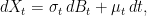(5)

the method can be applied. Now, the volatility in (3) is replaced by an average value across the interval (t_i-1, t_i).

The methods above are very useful, but there is a further improvement that can be made. Ideally, we would not have to specify an explicit value of the volatility σ. That is, it should be model independent. There are many reasons why this is desirable. Suppose that we are running a Monte Carlo simulation and generate samples of X at the times t_i. If the simulation only outputs values of X, then this is not sufficient to compute (3). So, it will be necessary to update the program running the simulation to also output the volatility. In some situations this might not be easy. For example, X could be a complicated function of various other processes and, although we could use Ito’s lemma to compute the volatility of X from the other processes, it could be messy. In some situations we might not even have access to the volatility or any method of computing it. For example, the values of X could be computed from historical data. We could be looking at the probability of stock prices crossing a level by looking at historical close fixings, without access to the complete intra-day data. In any case, a model independent discrete barrier adjustment would make applying it much easier.

---

Removing Volatility Dependence

How can the volatility term be removed from adjustment (3)? One idea is to replace it by an estimator computed from the samples of X, such as

While this would work, at least for a constant volatility process, it does not meet the requirements. For a general Ito process (5) with stochastic volatility, using an estimator computed over the whole time interval [0, T] may not be a good approximation for the volatility at the time that the barrier is hit. A possible way around this is for the adjustment (3) applied at time t_i to only depend on a volatility estimator computed from samples near the time. This would be possible, although it is not clear what is the best way to select these times. Besides, an important point to note is that we do not need a good estimate of the volatility, since that is not the goal here.

As explained in the previous post, adjustment (3) works because it corrects for the expected overshoot when the barrier is hit. Specifically, at the first time for which M_i ≥ K, the overshoot is R = X_ti – K. If there was no adjustment then the overshoot is positive and the leading order term in the discrete barrier approximation error is proportional to 𝔼[R]. The positive shift added to X_ti is chosen to compensate for this, giving zero expected overshoot to leading order, and reducing the barrier approximation error. The same applies to any similar adjustment. As long as there is sufficient freedom in choosing M_i, then it should be possible to do it in a way that has zero expected overshoot. Taking this to the extreme, it should be possible to compute the adjustment at time t_i using only the sampled values X_ti-1 and X_ti.

Consider adjustments of the form

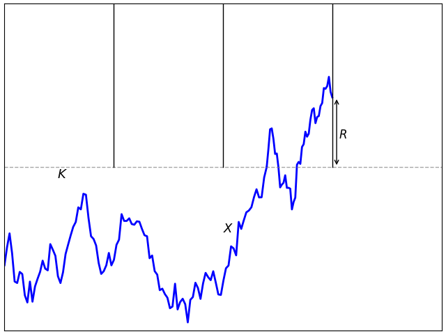
for θ: ℝ² → ℝ. By model independence, if this adjustment applies to a process X, then it should equally apply to the shifted and scaled processes X + a and bX for constants a and b > 0. Equivalently, θ satisfies the scaling and translation invariance,

(6)

This restricts the possible forms that θ can take.

Lemma 1 A function θ: ℝ² → ℝ satisfies (6) if and only if

for constants p, c.

Proof: Write θ(0, u) as the sum of its antisymmetric and symmetric parts

By scaling invariance, the first term on the right is proportional to u and the second is proportional to |u|. Hence,

for constants p and c. Using translation invariance,

as required. ⬜

I will therefore only consider adjustments where the maximum of the process across the interval (t_i-1, t_i) is replaced by

(7)

According to (3), the barrier condition sup_t≤TX_t ≥ K is replaced by the discrete approximation max_iM_i ≥ K.

There are various ways in which (7) can be parameterized, but this form is quite intuitive. The term pX_ti + (1 - p)X_ti-1 is an interpolation of the path of X, and c|X_ti – X_ti-1| represents a shift proportional to the sample deviation across the interval replacing the σ√δt term of the simple shift (3). The purpose of this post is to find values for p and c giving a good adjustment, improving convergence of the discrete approximation.

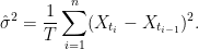
The discrete barrier condition M_i ≥ K given by (7) can be satisfied while the process is below the barrier level, giving a negative barrier ‘overshoot’ R = X_ti – K as in figure 2. As we will see, this is vital to obtaining an accurate approximation for the hitting probability.

---

Zero Expected Overshoot

When a continuous process X starting below K first satisfies the barrier condition X_t ≥ K then, by continuity, it will exactly equal K. However, when a discrete approximation to the barrier condition is first satisfied, this will not be true. The difference R = X_t – K at this time is known as the excess or overshoot. See figure 1 above. The leading order effect of this is to shift the barrier by an amount R and, to get a good approximation, we would want to make this expected overshoot equal to 0. There is a well-defined overshoot independent of the path of X in the limit as the sampling width goes to zero. Compare with theorem 3 of the previous post.

Theorem 2 Let X be Brownian motion with constant volatility σ > 0 and drift μ, and K > X₀ be a fixed level. For constants p, c and sampling times t_i = iδt, consider the adjustment M_i defined by (7) and let

be the discrete hitting time. Then the overshoot is R = X_τ – K.

As δt tends to zero, the normalized excess R/(σ√δt) converges to a limiting distribution independent of X. This distribution does not depend on σ, μ, K and has a finite mean β(p, c).

I will not prove this here, but will give a brief explanation of how it can be done. A Girsanov transformation reduces it to the case of zero drift and, then, scaling invariance reduces it to the case of unit volatility, σ = 1. It can also be shown that, in the limit, the discrete hitting time approaches the continuous one when X first hits level K. Hence, in the limit, the overshoot only depends on the path of X in an arbitrarily small neighborhood of this hitting time and, by independent increments of Brownian motion, will be independent of the path of X outside of this arbitrarily small interval.

By scaling invariance, again, the Brownian motion X can be replaced by B_t = (X_tδt - K)/√δt. The existence of the limit in theorem 2 is equivalent to saying that the overshoot of B when it reaches 0 converges to a limit in distribution as B₀ → -∞. However, this can be proved by coupling. Starting two independent Brownian motions far away from 0 and setting them to be equal after the time that they first coincide, they will be equal with high probability when the barrier is hit and, hence, they have the same overshoot with high probability. So, the overshoot converges to a limit as the initial state is moved far from the barrier level.

The expected overshoot β(p, c) effectively shifts the continuous barrier. Compare the following with conjecture 4 of the previous post.

Conjecture 3 Let X be Brownian motion with constant volatility σ > 0 and drift μ. For fixed positive time T and integer n, consider the sampling width δt = T/n and times t_i = iδt and let M_i be the discrete adjustment (7) for constants p, c. Then, for positive barrier K > X₀ define the shifted level

We have

as n → ∞ for any sufficiently regular function f: ℝ → ℝ.

As in the previous post, I do not prove this and it is not clear what ‘sufficiently regular’ should mean, although piecewise differentiable with reasonable growth bounds seems to be sufficient. The idea is that, by using M_i for the barrier condition rather than X_ti, the overshoot can be both positive or, as in figure 2 above, it can be negative. Choosing the parameters p and c carefully then, it is possible to ensure that the expected overshoot is zero. This results in an accurate approximation for the barrier hitting probability.

Corollary 4 With the notation of conjecture 3, we suppose that constants p, c are chosen such that β(p, c) = 0. Then,

as n → ∞.

To have a good discrete barrier approximation, we need the expected overshoot β(p, c) to be zero. Before solving for this, the following properties will be useful.

Lemma 5 The limiting expected overshoot satisfies

1. β(p, c) is monotonically decreasing from ∞ to -∞ as c increases from -∞ to ∞.
2. β(1 - p, c) = β(p, c).
3. β(p, c) is a function of p + c over the range p ≥ c and p + c ≥ 1.

Again, I will not go through the proof details here, but they are not too complicated. That β(p, c) is decreasing in c follows from the fact that M_i defined by (7) is explicitly increasing in c, so increasing its value causes the discrete barrier condition to be satisfied earlier, decreasing the overshoot.

Symmetry under exchanging p and 1 – p follows from the fact that this is the same as exchanging X_ti-1 and X_ti in (7) or, equivalently, applying the discrete barrier condition to the process in reverse time, which does not impact the probability of hitting the barrier to leading order by time-reversal symmetry of Brownian motion.

The third condition follows from the fact that, when p ≥ c and p + c ≥ 1, the discrete barrier condition is equivalent to

We are free to choose whatever value of p we like and, then, for a good barrier approximation the value of c is uniquely determined by the requirement β(p, c) = 0.

Lemma 6 For each real value p there is a unique c satisfying β(p, c) = 0. Setting γ(p) = c defines a continuous function γ: ℝ → ℝ satisfying

1. γ(1 - p) = γ(p).
2. γ(1/2) > 1/2.
3. γ(p) = 2p₀ – p for all p ≥ p₀, for some constant p₀ > 12 .

Proof: The existence of a unique value of c follows immediately from the first statement of lemma 5, and the identity γ(1 - p) = γ(p) follows from the second. Continuity follows from the fact that if p is changed by a small amount, then this does not affect the first time at which the barrier condition is satisfied, except with small probability.

Taking p = c = 1/2 gives the barrier condition M_i = max(X_ti-1, X_ti) and, so, the first time that M_i ≥ K is also the first time at which X_ti ≥ K. The expected overshoot is the same as for the unadjusted discrete barrier, which is nonnegative. Specifically, β(1/2, 1/2) ≈ 0.5826 and γ(1/2) > 1/2 as claimed.

Next, let p₀ ≥ 1/2 be the smallest value for which γ(p) ≤ p. This must exist since, for extremely large p values, even with c = 0 the value of M_i = X_ti-1 + p(X_ti - X_ti-1) will be large for relatively small increments of the process. So the adjusted barrier condition will be satisfied while X is still far from the barrier, giving a large negative overshoot. In that case, γ(p) < 0 < p, so p₀ exists. By the second statement of the lemma, p₀ > 1/2 and, by the intermediate value theorem, γ(p₀) = p₀.

If, for any p ≥ p₀, we set c = 2p₀ – p then p + c = 2p₀ > 1 independently of the choice of p, and p ≥ c. Lemma 5 tells us that β(p, c) is equal to β(p₀, p₀) = 0, proving that γ(p) = 2p₀ – p as required. ⬜

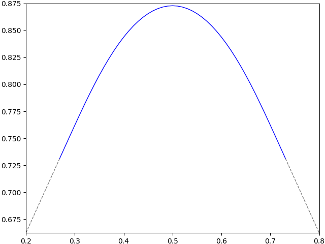
I numerically computed the function γ on a grid, and the results are shown in figure 3 below. Symmetry about p = 1/2 is clear. The critical value was computed as p₀ ≈ 0.7311. Beyond this γ(p) is linear and equal to 2p₀ – p as noted by lemma 6. Furthermore, p + c ≥ 1 and p ≥ c, so the discrete barrier adjustment is identical for all values in this range. Hence, the region p > p₀ is not interesting and is shown with a dashed line in the plot.

Tabulated values are displayed to 4 decimal places in figure 4 below, with each cell giving the value of c corresponding to the sum of the row and column p values. These extend to p < 0.5 by symmetry and to p > 0.79 by linear extrapolation. Values were computed using a grid as explained later.

p	.00	.01	.02	.03	.04	.05	.06	.07	.08	.09
0.5	.8729	.8726	.8717	.8703	.8682	.8656	.8624	.8586	.8543	.8493
0.6	.8438	.8378	.8312	.8241	.8165	.8084	.7998	.7908	.7815	.7720
0.7	.7622	.7522	.7423	.7323	.7223	.7123	.7023	.6923	.6823	.6723

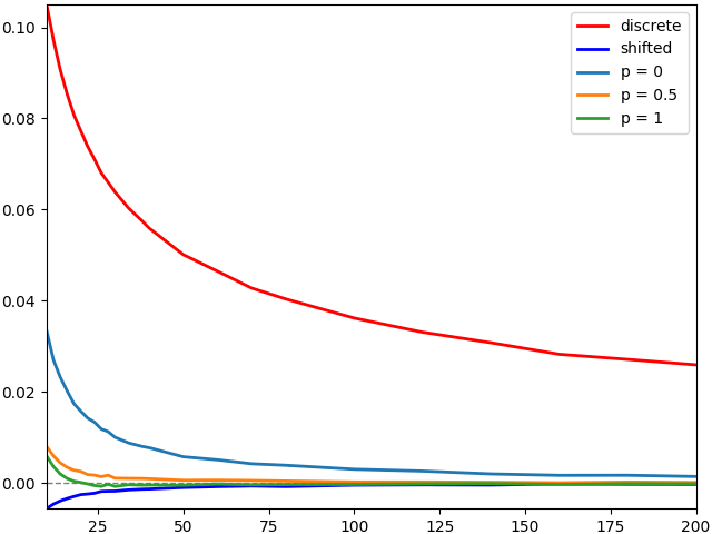
As a test of the convergence, I compute the difference between the probability of hitting a continuous barrier and that of hitting a discrete barrier. This uses 1 million Monte Carlo simulations so that the noise is within the line width of the plot. A volatility of 1 is used, so that it is standard Brownian motion, a terminal time T = 1, and barrier level K = 66%, so that the probability of hitting the continuous barrier is close to 50%. The difference between the continuous barrier probability and the discrete one is shown in figure 5 as a function of the number of sampling times. Five different discrete sampling approaches were used — unadjusted, the simple shift, and the adjustment described in this post for values of p equal to 0, 0.5 and 1. Explicitly, these use the following respective values for the maximum across each time step:

The results are shown in figure 5, showing the error versus the number of sampling times used. We see that all of the adjusted discrete approximations perform much better than the naive unadjusted discrete barrier, with a smaller error and converging faster. Also, for the model-independent method, the larger values of p perform best.

In order to scale the graph to better see the plots for the various discrete barrier adjustments, figure 6 shows the error for these on a larger scale. To further reduce noise, 10 million Monte Carlo paths were used.

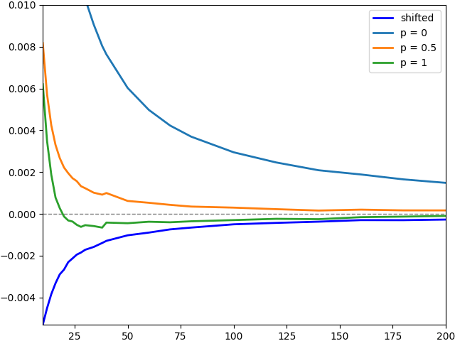
The results show that the adjustments for p = 0.5 and p = 1 perform about as well as the simple barrier shift and, for p = 1, it even looks a bit better. Which value works best in practice will likely depend on the use case, although the evidence suggests that any p ≥ 1/2 is a good choice.

Finally for this section I note that, although the theory above was based on X being Brownian motion with constant volatility and drift, it applies much more generally. Any Ito process (5) with piecewise continuous volatility and drift should also work, since such processes can be locally approximated with constant volatility and drift. Furthermore, as the adjustment (7) makes no reference to σ or μ, it carries across unchanged to the more general situation. This means that if we are able to simulate X at the sampling times, then the adjustment can be applied without requiring further information about the process.

---

Computing the Overshoot

Figures 2 and 3 showed the values of p and c such that the expected overshoot β(p, c) is zero. I now briefly explain how β(p, c) is computed. If X is a standard Brownian motion with volatility σ and zero drift, and K is the barrier level with sample spacing δt, consider

This is a random walk with standard normal increments and initial condition (K - X₀)/(σ√δt). We need to compute the expected overshoot as Y₀ goes to infinity. The barrier condition M_i ≥ K can be rearranged in terms of Y_i as

for constants a = 1 – 1/(p + c) and, if c > p, then b = 1 + 1/(c - p) otherwise b = ∞. In case the barrier condition is satisfied, the normalized overshoot is –Y_i. So, letting f(y) be the expected overshoot for initial condition Y₀ = y then the recurrence relation

holds, where N is normal with variance 1 and mean y. This is of the form

for linear operator L and function g which can be computed explicitly. This is solved by

I numerically represent f on a finite grid of y-values, in a range from 0 up to a maximum number of standard deviations. Then, L is represented by a matrix and the linear equation can be solved by standard methods. In practice, a maximum value of y = 8 and 1,000 grid points seems to work well. The values of f should flatten out to a constant for large values of y, which is the required value of β(p, c).

To demonstrate, I plot the results for various values of p in figure 7 below, with c chosen by bisection to make β(p, c) equal to zero within numerical accuracy. Also included is the result for a simple barrier shift of 0.5826 for comparison.

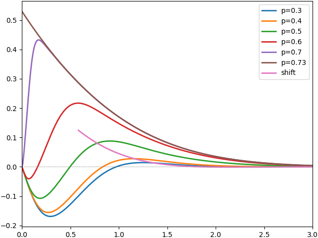
We see that the expected overshoot is not zero for initial condition close to the barrier but, once we are 3 standard deviations away, it has already converged close to zero.