Tomaszewski’s Conjecture

In a 1986 article of The American Mathematical Monthly written by Richard Guy, the following question was asked, and attributed to Bogusłav Tomaszewski: Consider n real numbers a₁, …, a_n such that Σ_ia_i² = 1. Of the 2ⁿ expressions |±a₁±⋯±a_n|,

A cursory attempt to find such real numbers a_i where more of the absolute signed sums have value  > 1 than have value  ≤ 1 should be enough to convince you that it is, in fact, impossible. The answer was therefore expected to be no, it is not possible. This has claim since been known as Tomaszewski’s conjecture, and there have been many proofs of weaker versions over the years until, finally, in 2020, it was proved by Keller and Klein in the paper Proof of Tomaszewski’s Conjecture on Randomly Signed Sums.

An alternative formulation is in terms of Rademacher sums

(1)

where X₁, …, X_n are independent ‘random signs’. That is, they have the Rademacher distribution ℙ(X_i = 1) = ℙ(X_i = -1) = 1/2. Then, Z has variance Σ_ia_i² and each of the 2ⁿ values ±a₁±⋯±a_n occurs with equal probability. So, Tomaszewski’s conjecture is the statement that

(2)

for unit variance Rademacher sums Z. It is usually stated in the equivalent, but more convenient form

(3)

I will discuss Tomaszewski’s conjecture and the ideas central to the proof given by Keller and Klein. I will not give a full derivation here. That would get very tedious, as evidenced both by the length of the quoted paper and by its use of computer assistance. However, I will prove the ‘difficult’ cases, which makes use of the tricks essential to Keller and Klein’s proof, with all remaining cases being, in theory, provable by brute force. In particular, I give a reformulation of the inductive stopping time argument that they used. This is a very ingenious trick that was introduced by Keller and Klein, and describing this is one of the main motivations for this post. Another technique also used in the proof is based on the reflection principle, in addition to some tricks discussed in the earlier post on Rademacher concentration inequalities.

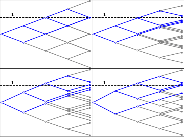
To get a feel for Rademacher sums, some simple examples are shown in figure 1. I use the notation a = (a₁, …, a_n) to represent the sequence with first n terms given by a_i, and any remaining terms equal to zero. The plots show the successive partial sums for each sequence of values of the random signs (X₁, X₂, …), with the dashed lines marking the ±1 levels.

The examples demonstrate that ℙ(|Z| ≤ 1) can achieve the bound of 1/2 in some cases, and be strictly more in others. The top-left and bottom-right plots show that, for certain coefficients, |Z| has a positive probability of being exactly equal to 1 and, furthermore, the claimed bound fails for ℙ(|Z|< 1). So, the inequality is optimal in a couple of ways. These examples concern a small number of nonzero coefficients. In the other extreme, for a large number of small coefficients, the central limit theorem says that Z is approximately a standard normal and ℙ(|Z| ≤ 1) is close to Φ(1) – Φ(-1) ≈ 0.68.

There is no reason for us to restrict to finite Rademacher sums, and (1) can be replaced by the infinite sum

where X₁, X₂, … are independent Rademacher random variables. This converges almost surely as long as σ² = Σ_ia_i² is finite, in which case Z has variance σ². Clearly, finite sums are just a special case of this where all but finitely many of the a_i are equal to zero. In the other direction, infinite sums can be approximated by finite ones. So, for the truth of the conjecture, it does not matter which is used. It is often notationally convenient to use infinite Rademacher sums.

The conjecture holds in the more symmetric form,

(4)

While this is stronger than (1), it is not difficult to show that they are equivalent. If (1) is known to hold, then we can consider applying it to Z′= uY + vZ where Y is a Rademacher variable independent of Z and u² + v² = 1. This is again a Rademacher sum of unit variance and, using the fact that Y has the same sign as Z with probability 1/2,

(5)

where η = √(1 - u)/(1 + u). If (1) holds, then the left hand side is bounded below by 1/2 and, letting u decrease to 0, then η → 1 and the right hand side tends to the left of (4).

The version of the conjecture (4) rearranges in the explicitly symmetric form

or, by subtracting ℙ(|Z|= 1) from both sides,

These forms of the conjecture are apparently stronger and more symmetric than that given by (2).

Another, seemingly even stronger version of the conjecture is

(6)

for any positive real η. This clearly implies the forms described above by taking η = 1. In the other direction, (5) can again by applied to give

for η ≤ 1 and, by symmetry, also for η ≥ 1. Rearranging,

Taking the limit of an increasing sequence of values for η converts the inequalities in the probabilities to their strict versions, giving (6).

Moving on to the proof overview, the first thing we can do is to assert that the coefficients are nonnegative and decreasing,

(7)

This does not lose generality, since we can always flip the signs and reorder the coefficients without impacting the distribution of Z. From here on, it will be assumed that (7) holds throughout. For brevity, I will write a numeral with an integer subscript k to refer to that value repeated k times so that, for example, (1₄) represents the sequence (1, 1, 1, 1). The proof, then, relies on splitting the domain for the coefficients a into several subdomains, and applying a different technique on each.

• Prove the case with a₁ + a₂ ≥ 1 using the inductive stopping time argument. This covers all cases with equality ℙ(|Z| ≤ 1) = 1/2.
• Prove for a neighbourhood of a = (1). This makes use of ‘local’ concentration inequalities bounding the probability of being in an interval by the probability of being in a separate interval, which can be proven by the reflection principle.
• Prove for neighbourhoods of a = (1₄)/2 and a = (1₉)/3. This uses the ideas discussed in the previous post on Rademacher concentration inequalities.
• Prove all other cases, which satisfy the strict bound ℙ(|Z|< 1) > 1/2, and can be done by brute force.

The first step mentioned, for a₁ + a₂ ≥ 1, not only makes use of the ingenious stopping time argument, but also includes all situations for which ℙ(|Z| ≤ 1) is exactly equal to 1/2. This is important because such cases are otherwise hard to handle since, in principle, an arbitrarily small bump to the coefficients could be enough to violate the claimed bound, and using approximations would not be sufficient to prove the claim.

The next two steps look at the finite set of ‘critical’ or ‘hard’ points. These are coefficients for which ℙ(|Z|< 1) is strictly less than 1/2. The conjecture only holds for such cases because there is a sufficiently large probability that |Z| is exactly equal to 1. Figure 2 lists these critical points along with the probabilities that |Z| is strictly and non-strictly less than 1. These are also displayed to several decimal places for easy comparison with the lower bound of 0.5.

a	ℙ(|Z|< 1)		ℙ(|Z| ≤ 1)
(1)	0	0.000	1	1.00
(14)/2	3/8	0.375	7/8	0.88
(19)/3	63/128	0.492	105/128	0.82

Methods based on approximations tend to break down in a neighbourhood of such critical points, so special handling is required. By ‘neighbourhood’, I mean all coefficient series whose terms are within a threshold δ > 0 of the critical values.

The final step is to prove the bound in all cases not covered by the first few steps. This can be done since, here, ℙ(|Z|< 1) is strictly greater than 1/2. As the bound is strict, approximations work well and, by continuity, the inequality automatically extends to a neighbourhood of any point a. See the discussion of compactness in the previous post — a brute force method of approximating the sum in a neighbourhood of a finite set of points will, in principle, suffice to prove it on the entire domain.

Of course, using further tricks will reduce the numerical work further, as is done by Keller and Klein. As this post is not intended to be a complete proof, I do not attempt this here. I will, however, briefly mention the use of Berry–Esseen for small values of a₁. Recall from the post on Rademacher concentration inequalities that this says that

for a fixed constant C and the standard normal distribution function Φ. It is known that C = 0.56 works (Shevstova, 2010). Hence, the conjectured bound ℙ(Z > 1) ≤ 1/4 follows so long as a₁ ≤ (1/4 - Φ(-1))/0.56, or a₁ ≤ 0.16. In their proof, Keller and Klein use a refinement of the Berry–Esseen theorem based on a method of Prawitz to significantly improve this to a₁ ≤ 0.31.

---

Induction for a₁ + a₂ ≥ 1

I work with infinite Rademacher sums with coefficients that are nonnegative and decreasing (7). Although using infinite sequences is convenient, the induction step requires that only finitely many are nonzero. The method will be to split out the first two terms a₁, a₂ from the sum and, then, remove a random but positive number of the remaining coefficients. Adding back new coefficients b₁, b₂ to replace the first two that were removed, we obtain Rademacher sums with strictly fewer nonzero terms. The induction shows that if Tomaszewski’s conjecture holds for these shorter sums, then it holds for the original one so long as a₁ + a₂ ≥ 1. The shorter sums need not satisfy b₁ + b₂ ≥ 1, meaning that the induction is not entirely self-contained. We still need to be able to prove the case for a₁ + a₂ < 1 by other methods. In the words of Keller and Klein, it is semi-inductive. By symmetry of the Rademacher distribution, the conjecture (3) is equivalent to

(8)

which is the form I will use here.

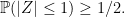
Moving on to describing the induction argument. based on that given by Keller and Klein, the explanation here is modified and reorganised to be easier to understand (to me) and is described by figure 3.

To start, use Z(n) to denote the partial sums,

The possible values of Z(2) are, in decreasing order of value,

The remaining terms in the partial sums are independent of Z(2) and will be denoted

for n ≥ 2. Adding this to the values of Z(2) gives the original Rademacher partial sums conditioned on the first two signs. I reflect Y(n) in the case that the first two signs are positive, which has no effect on the distribution since Y is symmetric and independent of Z(2).

These are the four blue paths shown in figure 3. So,

(9)

Reflecting Y(n) has the consequence that (Z₁(n) + Z₂(n))/2 = a₁ ≤ 1, meaning that whenever Z₁(n) ≥ 1 we also have Z_i(n) ≤ 1 for each i = 2, 3, 4.

Now, define N to be first time N > 2 at which Y(N) > 0 or equivalently Z₁(N) < z₁ (and set N = ∞ if this never happens). This is a random value and, in fact, is a stopping time under the filtration generated by X_i, since the event {N = n} only depends on the values of {X_i: i ≤ n}. Under the induction hypothesis that Tomaszewski’s bound (8) holds for all shorter sums, we prove that it must also hold for Z.

Start by conditioning on N = ∞. In that case, Z₁(n) ≥ 1 and, hence, Z_i(n) ≤ 1 for i = 2, 3, 4. So, only the i = 1 term in the sum on the right of (9) can be nonzero, giving the required upper bound of 1/4. The induction hypothesis was not required in this scenario.

Now, condition on N being a fixed finite value, and set h = Y(N) > 0. Consider the values

Defining b₁ = a₁ – h and b₂ = a₂ – h gives,

Furthermore, define

We can now construct new processes,

for n ≥ N. See figure 3.

Now, conditioned on N, Y(n) – Y(N) is the Rademacher sum a_N+1X_N+1 + ⋯+a_nX_n. Hence, if we let Z′ be the Rademacher sum with coefficients b = (b₁, b₂, a_N+1, a_N+2, …) then Z′+h conditioned on the first two signs has the same distribution as Z′_i(n) for large n. Comparing with (9),

(10)

We can compute the variance of Z′. This uses the fact that Σ_ia_i² = 1 and that h = Y(N - 1) + a_N ≤ a_N.

So, letting this variance be σ² then, if it is zero, the right hand side of (10) is zero. Otherwise,

This is bounded by 1/4 by the induction hypothesis, giving the claim.

The only place where a₁ + a₂ ≥ 1 was used is in the calculation of the variance of Z′, showing that it is bounded by (1 - h)² so that the induction hypothesis can be applied. We might think that a modified argument could be used in the case that a₁ + a₂ < 1. I have not been able to do this in such a way that Z′_i(n) ≥ Z_i(n) holds, as was required for (10), as well as making the variance of Z′ small enough for the induction hypothesis to apply. Also, Keller and Klein only use this induction for a₁ + a₂ ≥ 1, so it seems that they were also unable to make the approach work more generally.

---

Reflection Principle for a₁ ≈ 1

The first critical point to consider is the coefficient series a = (1). A neighbourhood of this consists of a such that a₁ is close to 1. To handle this, we split out the first term of the sum,

where Y is a Rademacher sum with unit variance and coefficients a_i+1/√1 - a₁². Then,

where η = √(1 - a₁)/(1 + a₁).We need to show that this is bounded by 1/2. This is reminiscent of (5) and can be rearranged similarly,

(11)

We prove that (11) holds for small η. As the case with a₁ + a₂ ≥ 1 was handled above, it is sufficient to consider a₁ + a₂ < 1 or, equivalently,

One method is to use Chebyshev’s inequality to bound the right hand side of (11) above by η². Using the method I will describe here, the left hand side can be shown to be bounded below by a multiple of η. So, (11) holds for sufficiently small η. Rather than separately bounding the two sides, it is more efficient to directly bound the left hand side by a multiple of the right side, which is the approach taken here.

Taking expectations of the inequality

(12)

immediately gives

This holds for all random variables with zero mean and unit variance, and is too weak for our purpose. The interval for Y on the left hand side needs to be shrunk to [-η, η]. This can be done with what Keller and Klein refer to as ‘local concentration inequalities’ which bound the probability of being in one interval by the probability of being in another. In fact, (11) is already a local inequality, as is the original statement (2) of the conjecture.

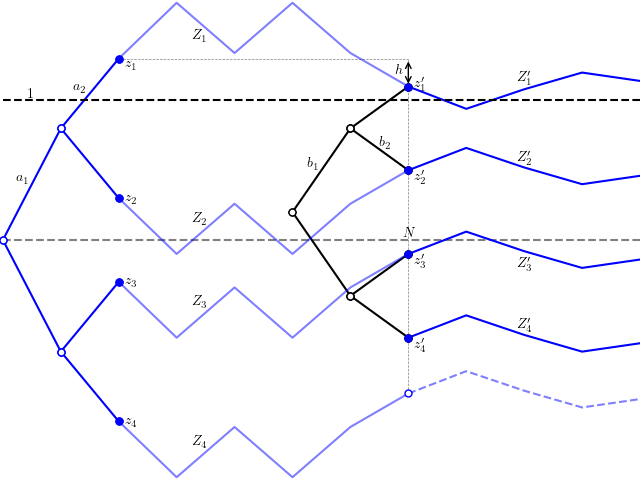
The trick which I describe to generate local concentration inequalities is the reflection principle. This enables us to map one interval into another in a measure-preserving way. Whereas with continuous processes such as standard Brownian motion, we can reflect it as soon as it hits a given level, for a discrete process such as the partial sums of a Rademacher series, we need to do this as soon as it crosses the level. As it will shoot slightly past the level before we have a chance to reflect, this overshoot affects the level of the reflected process. So, it is necessary to bound the Rademacher coefficients to ensure that this overshoot is small.

Lemma 1 For any x, u > 0 with x ≥ 2b₁, the inequality

holds.

Proof: Let Y(n) = b₁X₁ + ⋯+b_nX_n be the partial sums and N be the smallest positive integer such that Y(N) ≥ u/2. This is a random time and, in fact, is a stopping time. Consider the reflected process

As N is a stopping time, symmetry of the Rademacher distribution says that Y′(n) has the same distribution as Y(n). Furthermore, for N < ∞,

So, for any n ≥ N,

We have that Y′= Y(∞) has the same distribution as Y and, if Y ∈ [u, u + x] then n ≥ N and –x ≤ Y′ ≤ x.

⬜

The restriction b₁ ≤ x/2 is a bit too strong for our purposes. Fortunately, it is possible to relax this to b₁ ≤ x at the expense of a factor of 2 in the inequality.

Lemma 2 For any u ≥ x ≥ b₁, the inequality

holds.

Proof: Write Y = ±b₁ + Y′ for a Rademacher sum Y′ independent of the first sign, with coefficients (b₂, b₃, …). As this has the same distribution as ±(b₁ + Y′),

for y = x + b₁ ≥ 2b₁, with the final inequality using symmetry of Y′. Similarly,

with the final inequality using lemma 1. Combining the inequalities above gives the result. ⬜

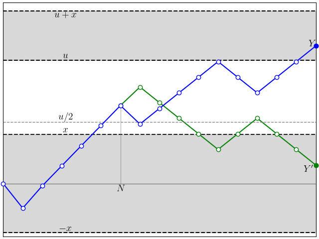
Now, for any x ≤ 1 ≤ y, we can improve on (12) by approximating 1 – Y² from above on a series of intervals. See figure 5.

(13)

Assuming that b₁ ≤ x, taking expectations of (13) and using 𝔼[Y²] = 1,

Lemma 2 bounds the individual probabilities in the sum,

Applying this over i ≥ 1 results in the local concentration bound

(14)

Using x = η and y = η^-1, the conjectured bound (11) holds so long as A(η) ≤ B(η^-1). It can be seen that this holds for η ≤ 0.437. In fact, for all η < 0.5 the sum (14) defining A(η) only has a term for i = 1, so is equal to 5 – 4η² and A(η) = B(η^-1) gives a quadratic in η² so can be solved exactly. From the definition of η used in (11) we have a₁ = (1 - η²)/(1 + η²) proving Tomaszewski’s conjecture for a₁ ≥ 0.68.

Actually, Keller and Klein go a step further in their proof. An additional transformation is combined with the reflection principle to reduce the factor of 4 to 2 for the i = 1 term in the sum (14) defining A(x). This is a reflection of a single sign X_i in the Rademacher sum, called the ‘single coordinate flip’, which improves the range on which (11) holds to η ≤ 0.54 and proves Tomaszewski’s conjecture for a₁ ≥ 0.55.

---

The Critical Points (1₄)/2 and (1₉)/3

I now look at the critical points a = (1₄)/2 and a = (1₉)/3 which, as shown in figure 2 satisfy ℙ(|Z|< 1) < 1/2. In order for Tomaszewski’s conjecture to hold, there must be a positive probability of |Z| being exactly equal to 1. By (4),

Indeed, for a = (1₄)/2 then ℙ(|Z|= 1) is 1/2, which is strictly greater than 1/4 = 1 – 2ℙ(|Z|< 1). Similarly, for a = (1₉)/3, ℙ(|Z|= 1) is 21/64 which is strictly greater than 1/64 = 1 – 2ℙ(|Z|< 1).

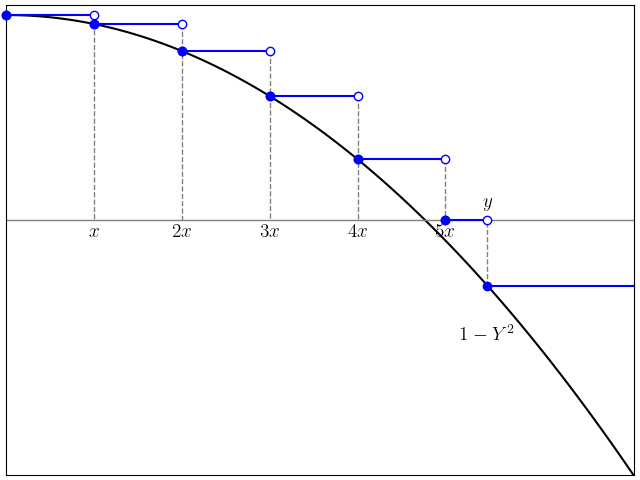
If the nonzero coefficients of a are bumped slightly, the values of Z will also be bumped. In order that the bound remains intact, sufficiently many of the states in which Z = 1 must be bumped to a value less than or equal to one. This is as shown in figure 6.

Neighbourhoods of these critical points can be handled using the methods described in the previous post on Rademacher concentration inequalities. As I will show, it is sufficient to find one or two pairs of bumped values of Z close to 1, each pair having average less than or equal to 1.

Suppose that Z is the Rademacher sum of length n with coefficients a. Then let Z′ be the same for coefficients a′, which are assumed close to a (and can have arbitrarily many nonzero values). We need to show that ℙ(|Z′| ≤ 1) ≥ 1/2 or, by symmetry, P(Z′ > 1) ≤ 1/4. The identity

holds for any pair of random variables. To show that the left hand side is bounded above by 1/4, it is enough to prove

(15)

Note that the final two terms only depend on a. For the critical point (1₄)/2 they give 1/16 and for (1₉)/3 they give 1/256.

Decompose Z′ as,

where Y is a unit variance Rademacher sum independent of Z and σ² = 1 – Σ_i≤n(a′_i)².

Next, let z_k (k = 1, …, m) be the finite sums a′₁s₁ + ⋯+a′_ns_n for signs s_i = ±1 such that the corresponding value Z = a₁s₁ + ⋯+a_ns_n is equal to 1. For a = (1₄)/2 these are the sums of a′_i with one minus sign, so and, for a = (1₉)/3, these are the sums with 3 minus signs, giving . I also set c = 2ⁿℙ(|Z| ≥ 1) – 2^n-2 so, with this notation, (15) is,

Taking c = 2ⁿℙ(|Z| ≥ 1) – 2^n-2, which gives c = 1 when a = (1₄)/2 and c = 2 for a = (1₉)/3,

(16)

In fact, the bound

(17)

is guaranteed to hold for a′ sufficiently close to the critical value a for each k = 1, …, m. To see why, note that as Z has a finite distribution, there exists a positive v such that Z < 1 – v whenever Z < 1. So, on the event Z′< 1 < Z we have Z′-Z > v and, again for a′ close enough to a, σY ≥ v. Also, for any positive u < v, we have z_k – 1 ≤ u for a′ close to a. This reduces (17) to showing that

Lemma 17 of the post on Rademacher concentration inequalities proved that this local concentration bound holds whenever σ is small enough, which will be the case if a′ is close to a. So, (16) reduces to proving that

(18)

for a′ close to a.

Now, as was shown in equation (12) of the post on Rademacher concentration inequalities,

holds whenever (z_j + z_k)/2 ≤ 1. This is simply using symmetry of the distribution of Y.

Hence, we obtain the following, using the notation of this section.

Lemma 3 If m > 2c and there exists at least c disjoint pairs i, j ∈ {1, …, m} with (z_i + z_j)/2 ≤ 1 then Tomaszewski’s conjecture holds for a′ in a neighbourhood of a.

As explained, this implies (18) for a suitable ordering of the z_k which, in turn, gives (16) and, then, gives ℙ(Z′ > 1) ≥ 1/4 as required. This may not be the most efficient method. Since the inequalities applied above may not be close to optimal, a more careful application of this method could be used to give reasonably large neighbourhoods to cover as much of the coefficient space as possible. However, the intent here is just to describe how Tomaszewski’s conjecture can be proven in principle without going through the full tedious calculations. It also shows why a bespoke method had to be used above for the critical point a = (1) since, there, m = 1 and there are not enough values z′_k lying close to 1 for the more generic method described here to work.

Now, suppose that a′_i = a_i + ϵ_i for i ≤ n and small bumps ϵ_i. As a_i are constant for the listed critical values and the coefficients can always be sorted into decreasing order, we suppose that the ϵ_i are decreasing in i. As they may be negative, they will likely not be decreasing in absolute value. In fact, the maximum absolute value of the ϵ_i is either |ϵ₁| or |ϵ_n|. Looking at the squared sum,

The critical values we are looking at have a_i constant and, so, Σ_iϵ_i < 0. Also, for each z_k we write

for signs s_i = ±1.

For the critical point a = (1₄)/2 the z_k are the sums of a′₁, a′₂, a′₃, a′₄ with one minus sign, so their average value is

So, with m = 4 and c = 1, the conditions of lemma 3 are satisfied and Tomaszewski’s conjecture holds in a neighbourhood of (1₄)/2.

For the critical point a = (1₉)/3 the z_k are the sums of a′_i with three minus signs. We can take,

Hence

The first inequality in each line just uses the condition that ϵ_i are decreasing in i. So, with m = 84 and c = 2, the conditions of lemma (3) are satisfied and Tomaszewski’s conjecture holds in a neighbourhood of a = (1₉)/3.