Stopping Times and the Debut Theorem

George Lowther Filtrations and Processes, Stochastic Calculus Notes 15 November 0928 February 23

In the previous two posts of the stochastic calculus notes, I began by introducing the basic concepts of a stochastic process and filtrations. As we often observe stochastic processes at a random time, a further definition is required. A stopping time is a random time which is adapted to the underlying filtration. As discussed in the previous post, we are working with respect to a filtered probability space ${(\Omega,\mathcal{F},\{\mathcal{F}_t\}_{t\ge 0},{\mathbb P})}$ .

Definition 1 A stopping time is a map ${\tau\colon\Omega\rightarrow{\mathbb R}_+\cup\{\infty\}}$ such that ${\{\tau\le t\}\in\mathcal{F}_t}$ for each ${t\ge 0}$ .

This definition is equivalent to stating that the process ${1_{[\tau,\infty)}}$ is adapted. Equivalently, at any time ${t}$ , the event ${\{\tau\le t\}}$ that the stopping time has already occurred is observable.

One common way in which stopping times appear is as the first time at which an adapted stochastic process hits some value. The debut theorem states that this does indeed give a stopping time.

Theorem 2 (Debut theorem) Let ${X}$ be an adapted right-continuous stochastic process defined on a complete filtered probability space. If ${K}$ is any real number then ${\tau\colon\Omega\rightarrow{\mathbb R}_+\cup\{\infty\}}$ defined by

$\displaystyle \tau(\omega)=\inf\left\{t\in{\mathbb R}_+\colon X_t(\omega)\ge K\right\}$ (1)

is a stopping time.

If ${\tau}$ is defined by equation (1) then it does seem intuitively obvious that it will be a stopping time. Clearly, ${\tau}$ will be less than or equal to ${t}$ precisely when ${X_s\ge K}$ for some ${s\le t}$ ,

$\displaystyle \left\{\tau\le t\right\}=\bigcup_{s\le t}\left\{X_s\ge K\right\}.$

(2)

As ${X}$ is an adapted process, each of the sets inside the union on the right hand side is ${\mathcal{F}_t}$ -measurable, and it seems reasonable to conclude that ${\{\tau\le t\}}$ should also be ${\mathcal{F}_t}$ -measurable, so that ${\tau}$ is a stopping time. However, the right hand side of (2) is an uncountable union, and sigma-algebras are only closed under countable unions and intersections in general. This result demonstrates the added difficulties in looking at continuous-time processes versus the discrete-time case. In discrete-time, the union in (2) is only over finitely many times and in that case the debut theorem follows easily.

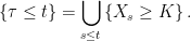
For continuous adapted processes (e.g. Brownian motion), the debut theorem is relatively easy to prove. Continuous processes always achieve their supremum value on any compact interval, and it is enough to look at the maximum process ${X^*_t=\sup_{s\le t}X_s}$ . By continuity, this supremum can be restricted to the countable set of rational numbers. Equation (2) reduces to the following,

$\displaystyle \left\{\tau\le t\right\}=\bigcap_{n=1}^\infty\bigcup_{s\in[0,t]\cap{\mathbb Q}}\left\{X_s\ge K-1/n\right\},$

which expresses ${\{\tau\le t\}}$ in terms of countable intersections of countable unions of ${\mathcal{F}_t}$ and hence is in ${\mathcal{F}_t}$ .

For right-continuous processes it is still true that ${X_t}$ is fully determined by its values at rational times, so it might seem that the debut theorem can be proved in a similar way as for continuous processes. However, this is not the case, and it is not possible to express ${\{\tau\le t\}}$ using countable unions and intersections of sets in ${\mathcal{F}_t}$ . In fact, ${\tau}$ need not be measurable in general, and the completeness of the filtered probability space is required. Still, it is not difficult to prove using only elementary techniques, and I give a proof of this below.

The debut theorem for right-continuous processes is only a special case of a more general result for arbitrary progressively measurable processes. However, the more general case relies on properties of analytic sets, which is a subject going well outside of these notes (I added a proof of the general case to PlanetMath), and right-continuous processes are more than general enough for these notes.

The value of a jointly measurable stochastic process at a random time is a measurable random variable, as mentioned in the previous post. As well as simply observing the value at this time, as the name suggests, stopping times are often used to stop the process. A process ${X}$ stopped at the random time ${\tau}$ is denoted by ${X^\tau}$ ,

$\displaystyle X^\tau_t(\omega)\equiv X_{t\wedge\tau(\omega)}(\omega).$

It is important that stopping an adapted process at a stopping time preserves the basic measurability properties.

Lemma 3 Let ${\tau}$ be a stopping time. If the stochastic process ${X}$ satisfies any of the following properties then so does the stopped process ${X^\tau}$ .

left-continuous and adapted.

right-continuous and adapted.

predictable.

optional.

progressively measurable.

Proof: First, recall that if ${X}$ is jointly measurable and ${\tau}$ is any random time then ${X_\tau}$ is measurable (see here). It follows from the decomposition

$\displaystyle X^\tau_t=1_{\{t\le\tau\}}X_t+1_{\{t>\tau\}}X_\tau.$

that ${X^\tau}$ is also jointly measurable. Now suppose that ${X}$ is progressive and ${T\ge 0}$ is any fixed time. By definition, ${X^T}$ is ${\mathcal{B}({\mathbb R}_+)\otimes\mathcal{F}_T}$ -measurable and, if ${\tau}$ is a stopping time, then ${\tau\wedge T}$ is ${\mathcal{F}_T}$ -measurable. Then, by what we have just shown above, the stopped process

$\displaystyle (X^\tau)^T=X^{\tau\wedge T}=(X^T)^{\tau\wedge T}$

is ${\mathcal{B}({\mathbb R}_+)\otimes\mathcal{F}_T}$ -measurable. This shows that ${X^\tau}$ is progressive.

Now let ${X}$ be left (resp. right) continuous and adapted. Then it is progressively measurable and, as has just been shown, ${X^\tau}$ is progressive. So, ${X^\tau}$ is adapted and it is clearly also left (resp. right) continuous.

Finally, we note that the collection of all processes ${X}$ such that ${X^\tau}$ is predictable (resp. optional) includes the left (resp. right) continuous adapted processes and is closed under the limit of a sequence of processes. So, by the functional monotone class theorem it follows that ${X^\tau}$ is predictable (resp. optional) whenever ${X}$ is predictable (resp. optional). ⬜

Other than the proof of the debut theorem given below, this covers the main results on stopping times for this post. All that remains are some very useful lemmas which are almost trivial to prove. First, it is often useful to replace the inequality ${\tau\le t}$ in the definition of a stopping time by a strict inequality. This can be done as long as the filtration is right-continuous.

Lemma 4 A map ${\tau\colon\Omega\rightarrow{\mathbb R}_+\cup\{\infty\}}$ is a stopping time with respect to the right-continuous filtration ${\{\mathcal{F}_{t+}\}_{t\ge 0}}$ if and only if ${\{\tau<t\}\in\mathcal{F}_t}$ for each ${t>0}$ .

Proof: For a stopping time ${\tau}$ using the fact that ${\mathcal{F}_{s+}\subseteq\mathcal{F}_t}$ for each ${s<t}$ gives

$\displaystyle \left\{\tau<t\right\}=\bigcup_{n=1}^\infty\left\{\tau\le t-1/n\right\}\in\mathcal{F}_t.$

Conversely, if ${\{\tau<t\}\in\mathcal{F}_t}$ for each time, then for any ${s>t}$ ,

$\displaystyle \left\{\tau\le t\right\}=\bigcap_{n=1}^\infty\left\{\tau< (t+1/n)\wedge s\right\}\in\mathcal{F}_s.$

As this is true for all ${s>t}$ it shows that ${\{\tau\le t\}\in\mathcal{F}_{t+}}$ . ⬜

Finally, the class of stopping times is closed under basic operations such as taking the maximum or minimum of two times or, for right-continuous filtrations, taking the limit of a sequence of times.

Lemma 5

If ${\sigma,\tau}$ are stopping times then so are ${\sigma\vee\tau}$ and ${\sigma\wedge\tau}$ .

Let ${\tau_n}$ be a sequence of stopping times converging to a limit ${\tau}$ and suppose that for each ${\omega\in\Omega}$ , ${\tau_n(\omega)\le\tau(\omega)}$ for large enough ${n}$ . Then ${\tau}$ is a stopping time. Note, in particular, that this includes the case where ${\tau_n}$ is increasing to the limit ${\tau}$ .

If ${\tau_n}$ is a sequence of stopping times then ${\sup_n\tau_n}$ is a stopping time.

If ${(\tau_n)_{n\in{\mathbb N}}}$ is a sequence of stopping times and the filtration is right-continuous, then ${\liminf_n\tau_n}$ and ${\limsup_n\tau_n}$ are stopping times.

Proof: If ${\sigma,\tau}$ are stopping times then

$\displaystyle \setlength\arraycolsep{2pt} \begin{array}{rl} &\displaystyle \left\{\sigma\vee\tau\le t\right\}=\left\{\sigma\le t\right\}\cap\left\{\tau\le t\right\}\in\mathcal{F}_t,\smallskip\\ &\displaystyle \left\{\sigma\wedge\tau\le t\right\}=\left\{\sigma\le t\right\}\cup\left\{\tau\le t\right\}\in\mathcal{F}_t. \end{array}$

So, ${\sigma\vee\tau}$ and ${\sigma\wedge\tau}$ are stopping times.

Now let ${\tau_n\rightarrow\tau}$ be a sequence of stopping times such that, for each ${\omega\in\Omega}$ , ${\tau_n(\omega)\le\tau(\omega)}$ for large ${n}$ . Then,

$\displaystyle \left\{\tau\le t\right\} = \bigcup_{n=1}^\infty\bigcap_{m=n}^\infty\left\{\tau_m\le t\right\}\in\mathcal{F}_t$

so that ${\tau}$ is a stopping time.

If ${\tau_n}$ is any sequence of stopping times then

$\displaystyle \left\{\sup{}_{\! n}\tau_n\le t\right\} = \bigcap_n\left\{\tau_n\le t\right\}\in\mathcal{F}_t,$

so ${\sup_n\tau_n}$ is a stopping time.

Finally, suppose that the filtration is right-continuous and that ${\tau_n}$ is a sequence of stopping times. Note that ${\liminf_n\tau_n<t}$ whenever ${\tau_n\le s}$ infinitely often for some ${s<t}$ , enabling us to write

$\displaystyle \left\{\liminf{}_{\! n}\tau_n<t\right\}=\bigcup_{k=1}^\infty\bigcap_{n=1}^\infty\bigcup_{m=n}^\infty\left\{\tau_m\le t-1/k\right\}\in\mathcal{F}_t.$

If the filtration is right-continuous, the lemma above shows that ${\liminf_n\tau_n}$ is a stopping time. Similarly, ${\limsup_n\tau_n<t}$ whenever ${\tau_n\le s}$ for all large ${n}$ and some ${s<t}$ giving

$\displaystyle \left\{\limsup{}_{\! n}\tau_n<t\right\}=\bigcup_{k=1}^\infty\bigcup_{n=1}^\infty\bigcap_{m=n}^\infty\left\{\tau_m\le t-1/k\right\}\in\mathcal{F}_t,$

so ${\limsup_n\tau_n}$ is also a stopping time. ⬜

Lemma 6 Let X be a cadlag adapted process. Then, there exists a sequence of stopping times ${\{\tau_n\}_{n=1,2,\ldots}}$ such that ${\tau_m\not=\tau_n}$ whenever ${m\not=n}$ and ${\tau_n < \infty}$ , and

$\displaystyle \left\{(t,\omega)\in{\mathbb R}_+\times\Omega\colon\Delta X_t(\omega)\not=0\right\}=\bigcup_{n=1}^\infty[\tau_n]$

Proof: For any positive real numbers ${s,\epsilon}$ define the random time

$\displaystyle \tau_{s,\epsilon}=\inf\left\{t\ge s\colon\vert\Delta X_t\vert > \epsilon\right\}.$

It can be seen that the union of the graphs ${[\tau_{s,\epsilon}]}$ over positive rationals ${s,\epsilon}$ is equal to the set of times at which ${\Delta X\not=0}$ so, to complete the proof of the lemma, it is enough to show that ${\tau_{s,\epsilon}}$ is a stopping time. That is, the set ${S=\{\tau_{s,\epsilon}\le t\}}$ is ${\mathcal{F}_t}$ -measurable. For ${t\le s}$ we have ${S=\emptyset}$ , so it is trivially measurable. So, we can suppose that ${t > s}$ . In that case, letting ${T}$ be any countable dense subset of ${[s,t]}$ with ${t\in T}$ , set

$\displaystyle U_n=\sup\left\{\lvert X_v-X_u\rvert \colon u,v\in T,\lvert v-u\rvert < 1/n\right\}.$

As this is the supremum of a countable set of ${\mathcal{F}_t}$ -measurable random variables, it is ${\mathcal{F}_t}$ -measurable. Also, using the cadlag property of ${X}$ ,

$\displaystyle \sup_{u\in(s,t]}\lvert \Delta X_u\rvert=\lim_{n\rightarrow\infty}U_n,$

so this is ${\mathcal{F}_t}$ -measurable. Then, ${\{\tau_{s,\epsilon} \le t\}}$ iff ${\sup_{u\in(s,t]}\lvert\Delta X_u\rvert > \epsilon}$ , which is ${\mathcal{F}_t}$ -measurable. ⬜

Proof of the debut theorem

I now give a proof of the debut theorem for a right-continuous adapted process ${X}$ . For a fixed real number ${K}$ , let ${\tau}$ be the first time at which ${X_\tau\ge K}$ . We need to show that this is a stopping time.

Given any stopping time ${\sigma\le\tau}$ , it is possible to define the larger time

$\displaystyle \sigma^+=\inf\left\{t\ge\sigma\colon\sup_{\sigma\le u\le t}X_u\ge K\right\}.$

Clearly, ${\sigma\le\sigma^+\le\tau}$ and it is easily seen that this is a stopping time. Indeed, ${\sigma^+}$ is less than or equal to a positive time ${t}$ precisely when, for each ${\epsilon>0}$ , there is a time ${s}$ in the range ${\sigma\le s\le t}$ satisfying ${X_s>K-\epsilon}$ . By right-continuity, it is enough to restrict to rational multiples of ${t}$ giving,

$\displaystyle \left\{\sigma^+\le t\right\}=\bigcap_{n=1}^\infty\bigcup_{a\in{\mathbb Q}\cap[0,1]}\left(\left\{\sigma\le at\right\}\cap\left\{X_{at}> K-1/n\right\}\right)\in\mathcal{F}_t.$

Also, using right continuity, ${\sigma^+}$ will be strictly greater than ${\sigma}$ whenever ${\sigma<\tau}$ .

The idea is to start with any stopping time bounded above by ${\tau}$ , for example ${\sigma=0}$ will do. Then, by iteratively replacing ${\sigma}$ by ${\sigma^+}$ , approach ${\tau}$ from below by successively closer approximations. Unfortunately, right-continuous processes can be badly behaved enough that this can fail, even after infinitely many steps, and transfinite induction would be required. A quicker approach, which I use here, is to make use of the idea of the essential supremum of a set of random variables.

Let ${\mathcal{T}}$ consist of the set of all stopping times ${\sigma}$ satisfying ${\sigma\le\tau}$ . By properties of the essential supremum, there exists a sequence ${\tau_n\in\mathcal{T}}$ such that ${\sigma=\sup_n\tau_n}$ is an essential supremum of ${\mathcal{T}}$ . As shown above, this is a stopping time and, therefore, ${\sigma\in\mathcal{T}}$ . The stopping time ${\sigma^+}$ defined above satisfies ${\sigma\le\sigma^+\le\tau}$ and is therefore in ${\mathcal{T}}$ . From the definition of the essential supremum, this implies that ${\sigma^+\le\sigma}$ and, therefore, ${\sigma^+=\sigma}$ with probability one. However, as mentioned above, ${\sigma^+>\sigma}$ whenever ${\sigma<\tau}$ , which therefore has zero probability.

We have shown that the stopping time ${\sigma}$ satisfies ${\sigma=\tau}$ almost surely. Finally, completeness of the filtered probability space implies that ${\tau}$ is a stopping time.

Published by George Lowther

View all posts by George Lowther

Published 15 November 0928 February 23

31 thoughts on “Stopping Times and the Debut Theorem”

Joseph says:

23 September 10 at 1:15 PM

With reference to your note on stopping times, I understand that if we consider a countable sequence of stopping times, then both the supremum and the infimum of such a sequence are stopping times. Now if we consider an uncountable sequence of stopping times. Is the supremum and infimum of this sequence a stopping time? If not, whats a counter-example? ( I am aware that the sigma algebra properties require countable unions and intersections )

Reply
1. George Lowther says:
  
  25 September 10 at 3:39 AM
  
  Hi. Counterexamples are,
  – Take your probability space to be the unit interval with the standard Lebesgue measure, A ⊂ [0,1] be a non-measurable set. Let τ_x(ω) be 1 if ω = x and 0 otherwise. This is a stopping time, but sup_x∈Aτ_x is 1 precisely on the non-measurable set A so is not a stopping time.
  – A more subtle example is that, on the space of cadlag processes (with the natural filtration), the first time τ at which which the coordinate process hits a level K is not a stopping time unless you complete the filtration (but it is the supremum of all stopping times T ≤ τ). This is harder to see though, but is true because the set {τ ≤ t} can be any analytic set, and need not be measurable (but is universally measurable).
  
  [Also, moved your comment to the relevant post]
  
  Reply
Jhonny says:

9 January 11 at 8:27 PM

According to the definition of stopping time, the most simple example of it would be T = c, c a real number, right?

Reply
1. George Lowther says:
  
  10 January 11 at 9:41 PM
  
  Right.
  
  Reply
Ilya says:

19 February 12 at 4:58 PM

Dear George, could you tell what does the notation $[\tau_n]$ means in the statement of Lemma 5? Also, in the last formula for $\{\sigma^\prime \le t\}$ should it be $\sigma^+$ ? I also have the following question: it seems that without an assumption on the completeness of the filtration we can at least state that there is a stopping time $\sigma$ such that the set $\{\sigma < \tau\}$ is a null set (not necessarily measurable). Is it right?

Reply
1. George Lowther says:
  
  22 February 12 at 1:51 AM
  
  – Yes, I seem to have used the notation $[\tau]$ without explaining what it means, which is a bit sloppy. It is standard notation though — it is a stochastic interval,
  
  $[\tau]=\left\{(t,\omega)\in\mathbb{R}_+\times\Omega\colon \tau(\omega)=t\right\}$
  
  You can think of $[\tau]$ as being a `random set’ $\{\tau(\omega)\}$ , which depends on $\omega$ .
  
  – I fixed the last formula. Thanks.
  
  – For your final question, yes. There will always be a stopping time $\sigma\le\tau$ with $\{\sigma <\tau\}$ being $\mathbb{P}$ -null.
  
  Reply
ben says:

24 October 12 at 4:29 AM

btw if you have two stopping times are their sum necessarily a stopping time?

Reply
1. George Lowther says:
  
  24 October 12 at 9:09 PM
  
  Yes. From an intuitive point of view, this seems obvious. Given that times σ, τ are observable when they occur, can you tell when σ + τ occurs? Yes, you clearly can, because σ and τ will both have already been observed by then.
  More precisely, given any measurable function f:R₊ → R₊ with f(s,t) ≥ max(s,t), then f(σ,τ) will be a stopping time whenever σ and τ are. In particular this holds for f(s,t) = s + t. More generally, you just need to require that f(s,t)∧u = f(s∧u,t∧u) holds.
  
  Reply
Ale says:

4 July 14 at 12:12 PM

Dear Almost Sure,

I thank you for your blog, it is very interesting and I’ve found here a lot of explanations. I’m reading the book “Stochastic calculus and financial applications” of Michael Steele and I have a doubt about the theorem “Doob’s Continuous-Time Stopping Theorem” on page 51. This is the statement: “Suppose {Mt} is a continuous martingale w.r.t. a filtration {Ft} that satisfies the usual conditions. If tau is a stopping time for {Ft}, the process Xt=M_min(t,tau) is also a continuous martingale w.r.t. {Ft}”

My doubt is about the condition that the filtration needs to satisfy the usual conditions. Your lemma 3 is a more general version of the theorem and you haven’t assumed the satisfation of the usual conditions. I don’t have very strong theoretical skills and so I’m worried that there is something that I don’t understand. In the proof of the theorem I am not able to find the place where the assumption is necessary. If you can give your opinion, I’ll appreciate it a lot. Thanks a lot

Reply
1. Ale says:
  
  4 July 14 at 1:29 PM
  
  Sorry, I read badly and your lemma 3 is not a generalization of the theorem “Continuous-time stopping theorem”. The lemma doesn’t assure the martingale property of the stopped process.
  
  Reply
2. George Lowther says:
  
  6 June 16 at 4:06 AM
  
  No, my Lemma 3 here does not involve martingales. However, I do prove the stopping theorem in a later post, and usual conditions are not required at all.
  
  Reply
Pingback: Proof of the Début theorem | Question and Answer
Ram says:

22 January 15 at 11:42 AM

Dear George, I am from engineering back ground. I see that when considering stopping times for continuous stochastic processes, you considered only over rational numbers. Also I see this in many texts when considering stopping time proof. I am quite confused about considring only rational numbers. Can you kindly clarify with some references also if possible.

Reply
1. George Lowther says:
  
  6 June 16 at 3:49 AM
  
  It is because in probability and measure theory, you can only work easily with operations on countably many sets (or events) at once. This is because of countable additivity of measure. Unions of uncountably many sets can give non-measurable sets. As the set of reals is uncountable, you need to restrict to a countable subset in many probabilistic arguments.
  
  Reply
  1. harfaw says:
    
    9 January 24 at 10:53 AM
    
    Regarding the uncountable union $\latex \cup_{s \leq t} \{K \leq X_s\}$ when $X$ is continuous, can we say that it includes all sample paths which cross $K$ at some time before $t$? In that case, we have $\latex \cup_{s \leq t} \{K \leq X_s\} = \{K \leq \max_{s \leq t} X_s\} = \{K \leq \sup_{s \leq t} X_s\} = \{K \leq \sup_{s \in [0, t] \cap \mathbb{Q}} X_s\}$. From here, I’m struggling to understand how to get $\latex \cap_{n \geq 1} \cup_{s \in [0, t] \cap \mathbb{Q}} \{K – 1/n \leq X_s\}$.
    
    Reply
Anonymous says:

19 June 16 at 11:56 PM

In the proof of lemma 5, you define a stopping time. But how do you know that what you define actually is a stopping time?

Reply
1. George Lowther says:
  
  20 June 16 at 12:37 AM
  
  You are right to ask – I did skip over the proof of that rather quickly. We need to show that $\{\tau_{s,\epsilon}\le t\}$ is $\mathcal{F}_t$ measurable. One way is is to set $U_n= \max\{X_u-X_v\colon u,v\in\mathbb{Q}\cap[s,t],\lvert u-v\rvert\le 1/n \}$ . Then, $\{\tau_{s,\epsilon}\le t\}$ iff $U_n > \epsilon$ eventually.
  
  Reply
  1. Anonymous says:
    
    9 August 16 at 4:52 PM
    
    Just one question regarding this, how are you allowed to use max, instead of sup? How do we know that the max exists?
    
    Reply
    1. George Lowther says:
      
      9 August 16 at 5:34 PM
      
      Actually, I should have written sup rather than max. I’ll update the post. The argument should be unchanged though. Actually, the max of $\Delta X$ does exist over any bounded innterval, but that is not important to the result.
2. George Lowther says:
  
  20 June 16 at 1:00 AM
  
  I updated the proof to include this argument.
  
  Reply
  1. Anonymous says:
    
    21 June 16 at 4:00 PM
    
    Thank you very much. I have been looking for arguments that jumps really are stopping times, and functions of jumps really are measurable etc.. Do you know if any book has these arguments? Or did you come up with it yourself? Anyway, great blog, really good work!
    
    Reply
    1. George Lowther says:
      
      26 July 16 at 9:26 PM
      
      It is quite standard, although the precise arguments in these notes are my own. I can check my references for published statements of such facts.
Pingback: Proof of Optional and Predictable Section | Almost Sure
Pingback: Martingale Inequalities | Almost Sure
Alex says:

2 March 20 at 4:52 AM

I’m struggling to understand the proof of Lemma 5.1 regarding

$\displaystyle \setlength\arraycolsep{2pt} \begin{array}{rl} &\displaystyle \left\{\sigma\vee\tau\le t\right\}=\left\{\sigma\le t\right\}\cap\left\{\tau\le t\right\}\in\mathcal{F}_t,\smallskip\\ &\displaystyle \left\{\sigma\wedge\tau\le t\right\}=\left\{\sigma\le t\right\}\cup\left\{\tau\le t\right\}\in\mathcal{F}_t. \end{array}$

Shouldn’t the set notations after the respective equal signs be reversed ?

Reply
1. George Lowther says:
  
  9 March 20 at 6:28 PM
  
  I think they are correct. As $\sigma\vee\tau$ is the maximum of $\sigma$ and $\tau$ , it is bounded above by t if and only if both of $\sigma$ and $\tau$ are.
  
  Reply
  1. Alex says:
    
    11 March 20 at 11:56 PM
    
    You are right. This notation (for minimum and maxmum) was new to me, but getting to know it makes it clear that your statements are true. Thank you for your answer (and your incredible blog!).
    
    Reply
Pingback: Proof of Début Theorem for right-continuous adapted process – Mathematics – Forum
ARS says:

25 February 23 at 11:46 AM

Hi! I think the last part of the first line after Definition 1 should read as: “ $\mathrm{1}_{[0,t]}\left(\tau(\cdot)\right)$ is adapted” instead of “ $\mathrm{1}_{[0,\tau]}$ is adapted”, right? That is, $X_t(\omega):=\mathrm{1}_{[0,t]}\left(\tau(\omega)\right)$ is adapted instead of $X_t(\omega)=\mathrm{1}_{[0,\tau(\omega)]}$ , which is time independent.

Reply
1. George Lowther says:
  
  28 February 23 at 2:00 AM
  
  actually, there was a typo which I fixed now. Maybe you misunderstand the notation. $X=1_{[\tau,\infty)}$ is equivalent to $X_t(\omega) = 1_{\tau(\omega)\le t}$ .
  
  Reply
  1. ARS says:
    
    28 February 23 at 8:04 AM
    
    Thanks for answering. The typo, [0, \tau] instead of [\tau,\infty), made me think that that particular notation was not being used! All clear then.
    
    Reply

	Anonymous on About
	Anonymous on About
	Anonymous on The Stochastic Integral
	Anonymous on Bessel Processes
	Anonymous on Bessel Processes
	Stat Prof on Pathwise Regularity of Optiona…
	Yang Chu on Spitzer’s Formula
	Anonymous on About
	Anonymous on Continuous Processes with Inde…
	Anonymous on Continuous Processes with Inde…

Proof of the debut theorem

Related

Published by George Lowther

31 thoughts on “Stopping Times and the Debut Theorem”

Leave a comment Cancel reply