The Kolmogorov Continuity Theorem

Fractional BM
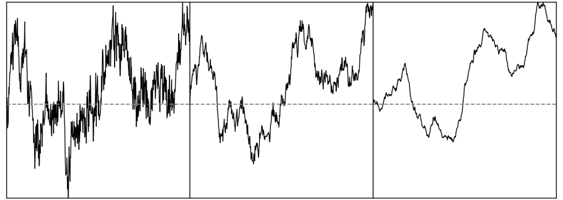
Figure 1: Fractional Brownian motion with H = 1/4, 1/2, 3/4

One of the common themes throughout the theory of continuous-time stochastic processes, is the importance of choosing good versions of processes. Specifying the finite distributions of a process is not sufficient to determine its sample paths so, if a continuous modification exists, then it makes sense to work with that. A relatively straightforward criterion ensuring the existence of a continuous version is provided by Kolmogorov’s continuity theorem.

For any positive real number {\gamma}, a map {f\colon E\rightarrow F} between metric spaces E and F is said to be {\gamma}-Hölder continuous if there exists a positive constant C satisfying

\displaystyle  d(f(x),f(y))\le Cd(x,y)^\gamma

for all {x,y\in E}. The smallest value of C satisfying this inequality is known as the {\gamma}-Hölder coefficient of {f}. Hölder continuous functions are always continuous and, at least on bounded spaces, is a stronger property for larger values of the coefficient {\gamma}. So, if E is a bounded metric space and {\alpha\le\beta}, then every {\beta}-Hölder continuous map from E is also {\alpha}-Hölder continuous. In particular, 1-Hölder and Lipschitz continuity are equivalent.

Kolmogorov’s theorem gives simple conditions on the pairwise distributions of a process which guarantee the existence of a continuous modification but, also, states that the sample paths {t\mapsto X_t} are almost surely locally Hölder continuous. That is, they are almost surely Hölder continuous on every bounded interval. To start with, we look at real-valued processes. Throughout this post, we work with repect to a probability space {(\Omega,\mathcal F, {\mathbb P})}. There is no need to assume the existence of any filtration, since they play no part in the results here

Theorem 1 (Kolmogorov) Let {\{X_t\}_{t\ge0}} be a real-valued stochastic process such that there exists positive constants {\alpha,\beta,C} satisfying

\displaystyle  {\mathbb E}\left[\lvert X_t-X_s\rvert^\alpha\right]\le C\lvert t-s\vert^{1+\beta},

for all {s,t\ge0}. Then, X has a continuous modification which, with probability one, is locally {\gamma}-Hölder continuous for all {0 < \gamma < \beta/\alpha}.

Continue reading “The Kolmogorov Continuity Theorem”

Local Martingales

Recall from the previous post that a cadlag adapted process {X} is a local martingale if there is a sequence {\tau_n} of stopping times increasing to infinity such that the stopped processes {1_{\{\tau_n>0\}}X^{\tau_n}} are martingales. Local submartingales and local supermartingales are defined similarly.

An example of a local martingale which is not a martingale is given by the `double-loss’ gambling strategy. Interestingly, in 18th century France, such strategies were known as martingales and is the origin of the mathematical term. Suppose that a gambler is betting sums of money, with even odds, on a simple win/lose game. For example, betting that a coin toss comes up heads. He could bet one dollar on the first toss and, if he loses, double his stake to two dollars for the second toss. If he loses again, then he is down three dollars and doubles the stake again to four dollars. If he keeps on doubling the stake after each loss in this way, then he is always gambling one more dollar than the total losses so far. He only needs to continue in this way until the coin eventually does come up heads, and he walks away with net winnings of one dollar. This therefore describes a fair game where, eventually, the gambler is guaranteed to win.

Of course, this is not an effective strategy in practise. The losses grow exponentially and, if he doesn’t win quickly, the gambler must hit his credit limit in which case he loses everything. All that the strategy achieves is to trade a large probability of winning a dollar against a small chance of losing everything. It does, however, give a simple example of a local martingale which is not a martingale.

The gamblers winnings can be defined by a stochastic process {\{Z_n\}_{n=1,\ldots}} representing his net gain (or loss) just before the n’th toss. Let {\epsilon_1,\epsilon_2,\ldots} be a sequence of independent random variables with {{\mathbb P}(\epsilon_n=1)={\mathbb P}(\epsilon_n=-1)=1/2}. Here, {\epsilon_n} represents the outcome of the n’th toss, with 1 referring to a head and -1 referring to a tail. Set {Z_1=0} and

\displaystyle  Z_{n}=\begin{cases} 1,&\text{if }Z_{n-1}=1,\\ Z_{n-1}+\epsilon_n(1-Z_{n-1}),&\text{otherwise}. \end{cases}

This is a martingale with respect to its natural filtration, starting at zero and, eventually, ending up equal to one. It can be converted into a local martingale by speeding up the time scale to fit infinitely many tosses into a unit time interval

\displaystyle  X_t=\begin{cases} Z_n,&\text{if }1-1/n\le t<1-1/(n+1),\\ 1,&\text{if }t\ge 1. \end{cases}

This is a martingale with respect to its natural filtration on the time interval {[0,1)}. Letting {\tau_n=\inf\{t\colon\vert X_t\vert\ge n\}} then the optional stopping theorem shows that {X^{\tau_n}_t} is a uniformly bounded martingale on {t<1}, continuous at {t=1}, and constant on {t\ge 1}. This is therefore a martingale, showing that {X} is a local martingale. However, {{\mathbb E}[X_1]=1\not={\mathbb E}[X_0]=0}, so it is not a martingale. Continue reading “Local Martingales”

Localization

Special classes of processes, such as martingales, are very important to the study of stochastic calculus. In many cases, however, processes under consideration `almost’ satisfy the martingale property, but are not actually martingales. This occurs, for example, when taking limits or stochastic integrals with respect to martingales. It is necessary to generalize the martingale concept to that of local martingales. More generally, localization is a method of extending a given property to a larger class of processes. In this post I mention a few definitions and simple results concerning localization, and look more closely at local martingales in the next post.

Definition 1 Let P be a class of stochastic processes. Then, a process X is locally in P if there exists a sequence of stopping times {\tau_n\uparrow\infty} such that the stopped processes

\displaystyle  1_{\{\tau_n>0\}}X^{\tau_n}

are in P. The sequence {\tau_n} is called a localizing sequence for X (w.r.t. P).

I write {P_{\rm loc}} for the processes locally in P. Choosing the sequence {\tau_n\equiv\infty} of stopping times shows that {P\subseteq P_{\rm loc}}. A class of processes is said to be stable if {1_{\{\tau>0\}}X^\tau} is in P whenever X is, for all stopping times {\tau}. For example, the optional stopping theorem shows that the classes of cadlag martingales, cadlag submartingales and cadlag supermartingales are all stable.

Definition 2 A process is a

  1. a local martingale if it is locally in the class of cadlag martingales.
  2. a local submartingale if it is locally in the class of cadlag submartingales.
  3. a local supermartingale if it is locally in the class of cadlag supermartingales.

Continue reading “Localization”

Class (D) Processes

A stochastic process X is said to be uniformly integrable if the set of random variables {\{X_t\colon t\in{\mathbb R}_+\}} is uniformly integrable. However, even if this is the case, it does not follow that the set of values of the process sampled at arbitrary stopping times is uniformly integrable.

For the case of a cadlag martingale X, optional sampling can be used. If {t\ge 0} is any fixed time then this says that {X_\tau={\mathbb E}[X_t\mid\mathcal{F}_\tau]} for stopping times {\tau\le t}. As sets of conditional expectations of a random variable are uniformly integrable, the following result holds.

Lemma 1 Let X be a cadlag martingale. Then, for each {t\ge 0}, the set

\displaystyle  \{X_\tau\colon\tau\le t\text{\ is\ a\ stopping\ time}\}

is uniformly integrable.

This suggests the following generalized concepts of uniform integrability for stochastic processes.

Definition 2 Let X be a jointly measurable stochastic process. Then, it is

  • of class (D) if {\{X_\tau\colon\tau<\infty\text{ is a stopping time}\}} is uniformly integrable.
  • of class (DL) if, for each {t\ge 0}, {\{X_\tau\colon\tau\le t\text{ is a stopping time}\}} is uniformly integrable.

Continue reading “Class (D) Processes”

U.C.P. and Semimartingale Convergence

A mode of convergence on the space of processes which occurs often in the study of stochastic calculus, is that of uniform convergence on compacts in probability or ucp convergence for short.

First, a sequence of (non-random) functions {f_n\colon{\mathbb R}_+\rightarrow{\mathbb R}} converges uniformly on compacts to a limit {f} if it converges uniformly on each bounded interval {[0,t]}. That is,

\displaystyle  \sup_{s\le t}\vert f_n(s)-f(s)\vert\rightarrow 0 (1)

as {n\rightarrow\infty}.

If stochastic processes are used rather than deterministic functions, then convergence in probability can be used to arrive at the following definition.

Definition 1 A sequence of jointly measurable stochastic processes {X^n} converges to the limit {X} uniformly on compacts in probability if

\displaystyle  {\mathbb P}\left(\sup_{s\le t}\vert X^n_s-X_s\vert>K\right)\rightarrow 0

as {n\rightarrow\infty} for each {t,K>0}.

Continue reading “U.C.P. and Semimartingale Convergence”

Martingale Inequalities

Martingale inequalities are an important subject in the study of stochastic processes. The subject of this post is Doob’s inequalities which bound the distribution of the maximum value of a martingale in terms of its terminal distribution, and is a consequence of the optional sampling theorem. We work with respect to a filtered probability space {(\Omega,\mathcal{F},\{\mathcal{F}_t\}_{t\ge 0},{\mathbb P})}. The absolute maximum process of a martingale is denoted by {X^*_t\equiv\sup_{s\le t}\vert X_s\vert}. For any real number {p\ge 1}, the {L^p}-norm of a random variable {Z} is

\displaystyle  \Vert Z\Vert_p\equiv{\mathbb E}[|Z|^p]^{1/p}.

Then, Doob’s inequalities bound the distribution of the maximum of a martingale by the {L^1}-norm of its terminal value, and bound the {L^p}-norm of its maximum by the {L^p}-norm of its terminal value for all {p>1}.

Theorem 1 Let {X} be a cadlag martingale and {t>0}. Then

  1. for every {K>0},

    \displaystyle  {\mathbb P}(X^*_t\ge K)\le\frac{\lVert X_t\rVert_1}{K}.

  2. for every {p>1},

    \displaystyle  \lVert X^*_t\rVert_p\le \frac{p}{p-1}\Vert X_t\Vert_p.

  3. \displaystyle  \lVert X^*_t\rVert_1\le\frac e{e-1}{\mathbb E}\left[\lvert X_t\rvert \log\lvert X_t\rvert+1\right].

Continue reading “Martingale Inequalities”

Martingale Convergence

The martingale property is strong enough to ensure that, under relatively weak conditions, we are guaranteed convergence of the processes as time goes to infinity. In a previous post, I used Doob’s upcrossing inequality to show that, with probability one, discrete-time martingales will converge at infinity under the extra condition of {L^1}-boundedness. Here, I consider continuous-time martingales. This is a more general situation, because it considers limits as time runs through the uncountably infinite set of positive reals instead of the countable set of positive integer times. Although these results can also be proven in a similar way by counting the upcrossings of a process, I instead show how they follow directly from the existence of cadlag modifications. We work with respect to a complete filtered probability space {(\Omega,\mathcal{F},\{\mathcal{F}_t\}_{t\ge 0},{\mathbb P})}.

Recall that a stochastic process {X} is {L^1}-bounded if the set {\{X_t\colon t\in{\mathbb R}_+\}} is {L^1}-bounded. That is, {{\mathbb E}|X_t|} is bounded above by some finite value as {t} runs through the positive reals.

Theorem 1 Let {X} be a cadlag and {L^1}-bounded martingale (or submartingale, or supermartingale). Then, the limit {X_\infty=\lim_{t\rightarrow\infty}X_t} exists and is finite, with probability one.

Continue reading “Martingale Convergence”

Optional Sampling

Doob’s optional sampling theorem states that the properties of martingales, submartingales and supermartingales generalize to stopping times. For simple stopping times, which take only finitely many values in {{\mathbb R}_+}, the argument is a relatively basic application of elementary integrals. For simple stopping times {\sigma\le\tau}, the stochastic interval {(\sigma,\tau]} and its indicator function {1_{(\sigma,\tau]}} are elementary predictable. For any submartingale {X}, the properties of elementary integrals give the inequality

\displaystyle  {\mathbb E}\left[X_\tau-X_\sigma\right]={\mathbb E}\left[\int_0^\infty 1_{(\sigma,\tau]}\,dX\right]\ge 0. (1)

For a set {A\in \mathcal{F}_\sigma} the following

\displaystyle  \sigma^\prime(\omega)=\begin{cases} \sigma(\omega),&\textrm{if }\omega\in A,\\ \tau(\omega),&\textrm{otherwise}, \end{cases}

is easily seen to be a stopping time. Replacing {\sigma} by {\sigma^\prime} extends inequality (1) to the following,

\displaystyle  {\mathbb E}\left[1_A(X_\tau-X_\sigma)\right]={\mathbb E}\left[X_\tau-X_{\sigma^\prime}\right]\ge 0. (2)

As this inequality holds for all sets {A\in\mathcal{F}_\sigma} it implies the extension of the submartingale property {X_\sigma\le{\mathbb E}[X_\tau\vert\mathcal{F}_\sigma]} to the random times. This argument applies to all simple stopping times, and is sufficient to prove the optional sampling result for discrete time submartingales. In continuous time, the additional hypothesis that the process is right-continuous is required. Then, the result follows by taking limits of simple stopping times.

Theorem 1 Let {\sigma\le\tau} be bounded stopping times. For any cadlag martingale, submartingale or supermartingale {X}, the random variables {X_\sigma, X_\tau} are integrable and the following are satisfied.

  1. If {X} is a martingale then, {X_\sigma={\mathbb E}\left[X_{\tau}\vert\mathcal{F}_\sigma\right].}
  2. If {X} is a submartingale then, {X_\sigma\le{\mathbb E}\left[X_{\tau}\vert\mathcal{F}_\sigma\right].}
  3. If {X} is a supermartingale then, {X_\sigma\ge{\mathbb E}\left[X_{\tau}\vert\mathcal{F}_\sigma\right].}

Continue reading “Optional Sampling”

Cadlag Modifications

As was mentioned in the initial post of these stochastic calculus notes, it is important to choose good versions of stochastic processes. In some cases, such as with Brownian motion, it is possible to explicitly construct the process to be continuous. However, in many more cases, it is necessary to appeal to more general results to assure the existence of such modifications.

The theorem below guarantees that many of the processes studied in stochastic calculus have a right-continuous version and, furthermore, these versions necessarily have left limits everywhere. Such processes are known as càdlàg from the French for “continu à droite, limites à gauche” (I often drop the accents, as seems common). Alternative terms used to refer to a cadlag process are rcll (right-continuous with left limits), R-process and right process. For a cadlag process {X}, the left limit at any time {t>0} is denoted by {X_{t-}} (and {X_{0-}\equiv X_0}). The jump at time {t} is denoted by {\Delta X_t=X_t-X_{t-}}.

We work with respect to a complete filtered probability space {(\Omega,\mathcal{F},\{\mathcal{F}_t\}_{t\ge 0},{\mathbb P})}.

Theorem 1 below provides us with cadlag versions under the condition that elementary integrals of the processes cannot, in a sense, get too large. Recall that elementary predictable processes are of the form

\displaystyle  \xi=Z_01_{\{t=0\}}+\sum_{k=1}^nZ_k1_{\{s_k<t\le t_k\}}

for times {s_k<t_k}, {\mathcal{F}_0}-measurable random variable {Z_0} and {\mathcal{F}_{s_k}}-measurable random variables {Z_k}. Its integral with respect to a stochastic process {X} is

\displaystyle  \int_0^t \xi\,dX=\sum_{k=1}^nZ_k(X_{t_k\wedge t}-X_{s_{k}\wedge t}).

An elementary predictable set is a subset of {{\mathbb R}_+\times\Omega} which is a finite union of sets of the form {\{0\}\times F} for {F\in\mathcal{F}_0} and {(s,t]\times F} for nonnegative reals {s<t} and {F\in\mathcal{F}_s}. Then, a process is an indicator function {1_A} of some elementary predictable set {A} if and only if it is elementary predictable and takes values in {\{0,1\}}.

The following theorem guarantees the existence of cadlag versions for many types of processes. The first statement applies in particular to martingales, submartingales and supermartingales, whereas the second statement is important for the study of general semimartingales.

Theorem 1 Let X be an adapted stochastic process which is right-continuous in probability and such that either of the following conditions holds. Then, it has a cadlag version.

  • X is integrable and, for every {t\in{\mathbb R}_+},

    \displaystyle  \left\{{\mathbb E}\left[\int_0^t1_A\,dX\right]\colon A\textrm{ is elementary}\right\}

    is bounded.

  • For every {t\in{\mathbb R}_+} the set

    \displaystyle  \left\{\int_0^t1_A\,dX\colon A\textrm{ is elementary}\right\}

    is bounded in probability.

Continue reading “Cadlag Modifications”

Upcrossings, Downcrossings, and Martingale Convergence

The number of times that a process passes upwards or downwards through an interval is refered to as the number of upcrossings and respectively the number of downcrossings of the process.

Upcrossings
A process with 3 upcrossings of the interval [a,b]

Consider a process {X_t} whose time index {t} runs through an index set {\mathbb{T}\subseteq{\mathbb R}}. For real numbers {a<b}, the number of upcrossings of {X} across the interval {[a,b]} is the supremum of the nonnegative integers {n} such that there exists times {s_k,t_k\in\mathbb{T}} satisfying

\displaystyle  s_1<t_1<s_2<t_2<\cdots<s_n<t_n (1)

and for which {X_{s_k}\le a<b\le X_{t_k}}. The number of upcrossings is denoted by {U[a,b]}, which is either a nonnegative integer or is infinite. Similarly, the number of downcrossings, denoted by {D[a,b]}, is the supremum of the nonnegative integers {n} such that there are times {s_k,t_k\in\mathbb{T}} satisfying (1) and such that {X_{s_k}\ge b>a\ge X_{t_k}}.

Note that between any two upcrossings there is a downcrossing and, similarly, between any two downcrossings there is an upcrossing. It follows that {U[a,b]} and {D[a,b]} can differ by at most 1, and they are either both finite or both infinite.

The significance of the upcrossings of a process to convergence results is due to the following criterion for convergence of a sequence.

Theorem 1 A sequence {x_1,x_2,\ldots} converges to a limit in the extended real numbers if and only if the number of upcrossings {U[a,b]} is finite for all {a<b}.

Continue reading “Upcrossings, Downcrossings, and Martingale Convergence”