Stochastic differential equations (SDEs) form a large and very important part of the theory of stochastic calculus. Much like ordinary differential equations (ODEs), they describe the behaviour of a dynamical system over infinitesimal time increments, and their solutions show how the system evolves over time. The difference with SDEs is that they include a source of random noise., typically given by a Brownian motion. Since Brownian motion has many pathological properties, such as being everywhere nondifferentiable, classical differential techniques are not well equipped to handle such equations. Standard results regarding the existence and uniqueness of solutions to ODEs do not apply in the stochastic case, and cannot readily describe what it even means to solve such as system. I will make some posts explaining how the theory of stochastic calculus applies to systems described by an SDE.
Consider a stochastic differential equation describing the evolution of a real-valued process {Xt}t≥0,
 |
(1) |
which can be specified along with an initial condition X0 = x0. Here, b is the drift specifying how X moves on average across the dt time, σ is a volatility term giving the amplitude of the random noise and W is a driving Brownian motion providing the source of the randomness. There are numerous situations where equations such as (1) are used, with applications in physics, finance, filtering theory, and many other areas.
In the case where σ is zero, (1) is just an ordinary differential equation dX/dt = b(X). In the general case, we can informally think of dividing through by dt to give an ODE plus an additional noise term
 |
(2) |
I have set ξt = dWt/dt which can be thought of as a process whose values at each time are independent zero-mean random variables. As mentioned above, though, Brownian motion is not differentiable so this does not exist in the usual sense. While it can be described by a kind of random distribution, even distribution theory is not well-equipped to handle such equations involving multiplying by the nondifferentiable process σ(Xt). Instead, (1) can be integrated to obtain
 |
(3) |
where the right-hand-side is interpreted using stochastic integration with respect to the semimartingale W. Likewise, X will be a semimartingale, and such solutions are often referred to as diffusions.
The differential form (1) can be interpreted as a shorthand for the integral expression (3), which I will do in these notes. It can be generalized to n-dimensional processes by allowing b to take values in ℝn, σ(x) to be an n × m matrix, and W to be an m-dimensional Brownian motion. That is, W = (W1, …, Wm) where Wi are independent Brownian motions. I will sometimes write this as
where the summation convention is being applied, with subscripts or superscripts occuring more than once in a single term being summed from 1 to n.
Unlike ODEs, when dealing with SDEs we need to consider what underlying probability space the solution is defined with respect to. This leads to the existence of different classes of solutions.
- Strong solutions where X can be expressed as a measurable function of the Brownian motion W or, equivalently, X is adapted to its natural filtration.
- Weak solutions where X need not be a function of W. Such cases may require additional randomness so may not exist on the probability space with respect to which the Brownian motion W is defined. It can be necessary to extend the filtered probability space to construct these solutions.
Likewise, when considering uniqueness of solutions, there are different ways this occurs.
- Pathwise uniqueness where, up to indistinguishability, there is only one solution X. This should hold not just on one specific space containing a Brownian motion W, but on all such spaces. That is, weak solutions should be unique.
- Uniqueness in law where there may be multiple pathwise solutions, but their distribution is uniquely determined by the SDE.
There are various general conditions under which strong solutions and pathwise uniqueness are guaranteed for SDE (1) , such as the Itô result for Lipschitz continuous coefficients. I covered this situation in a previous post.
Other than using the SDE (1), such systems can also be described by an associated differential operator. For the n-dimensional case set a(x) = σ(x)σ(x)T, which is an n × n positive semidefinite matrix. Then, the second order operator L can be defined
operating on twice continuously differentiable functions f: ℝn → ℝ. Being able to effortlessly switch between descriptions using the SDE (1) and the operator L is a huge benefit when working with such systems. There are several different ways in which the operator can be used to describe a stochastic process, all of which relate to weak solutions and uniqueness in law of the SDE.
Markov Generator: A Markov process is a weak solution to the SDE (1) if its infinitesimal generator is L. That is, if the transition function is Pt then,
for suitably regular functions f.
Backwards Equation: For a function f: ℝn × ℝ+ → ℝ, f(t, Xt) is a local martingale if and only if it solves the partial differential equation (PDE)
Consequently, for any time t > 0 and function g: ℝd → ℝ, if we let f be a solution to the PDE above with boundary condition f(x, t) = g(x) then, assuming integrability conditions, the conditional expectations at times s < t are
If the conditions are satisfied, this describes a Markov process and gives its transition probabilities, describing the distribution of X and implying uniqueness in law.
Forward Equation: Assuming that it is sufficiently smooth, the probability density p(t, x) of Xt satisfies the PDE
where LT is the transpose of operator L
If this PDE has a unique solution for given initial distribution, then this uniquely determines the distribution of Xt. So, if unique solutions to the forward equation exist starting at every future time, it gives uniqueness in law for X.
Martingale problem: Any weak solution to SDE (1) satisfies the property that
is a local martingale for twice continuously differentiable functions f: ℝn → ℝ. This approach, which was pioneered by Stroock and Varadhan, has many benefits over the other applications of operator L described above, since it applies much more generally. We do not need to a-priori impose any properties on X such as being Markov, and as the test functions f are chosen at will, they automatically satisfy the necessary regularity properties. As well as being a very general way to describe solutions to a stochastic dynamical system, it turns out to be very fruitful. The striking and far-reaching Stroock–Varadhan uniqueness theorem, in particular, guarantees existence and uniqueness in law so long as a is continuous and positive definite and b is locally bounded.


![{ Y={\mathbb E}[X\vert\mathcal F_t]}](https://s0.wp.com/latex.php?latex=%7B+Y%3D%7B%5Cmathbb+E%7D%5BX%5Cvert%5Cmathcal+F_t%5D%7D&bg=ffffff&fg=000000&s=0&c=20201002)
![{ Y^*={\mathbb E}[X^*\vert\mathcal F'_t]}](https://s0.wp.com/latex.php?latex=%7B+Y%5E%2A%3D%7B%5Cmathbb+E%7D%5BX%5E%2A%5Cvert%5Cmathcal+F%27_t%5D%7D&bg=ffffff&fg=000000&s=0&c=20201002)


![\displaystyle {\mathbb P}(A\cap B) = {\mathbb E}\left[{\mathbb P}(A\vert\mathcal K){\mathbb P}(B\vert\mathcal K)\right]](https://s0.wp.com/latex.php?latex=%5Cdisplaystyle+%7B%5Cmathbb+P%7D%28A%5Ccap+B%29+%3D+%7B%5Cmathbb+E%7D%5Cleft%5B%7B%5Cmathbb+P%7D%28A%5Cvert%5Cmathcal+K%29%7B%5Cmathbb+P%7D%28B%5Cvert%5Cmathcal+K%29%5Cright%5D+&bg=ffffff&fg=000000&s=0&c=20201002)


for all bounded
for all bounded
for all bounded


![\displaystyle {\mathbb E}[g(X_t)\;\vert\mathcal F_s]=f(X_s,s).](https://s0.wp.com/latex.php?latex=%5Cdisplaystyle+%7B%5Cmathbb+E%7D%5Bg%28X_t%29%5C%3B%5Cvert%5Cmathcal+F_s%5D%3Df%28X_s%2Cs%29.+&bg=ffffff&fg=000000&s=0&c=20201002)


![{[0,T]}](https://s0.wp.com/latex.php?latex=%7B%5B0%2CT%5D%7D&bg=ffffff&fg=000000&s=0&c=20201002) is continuous and equal to zero at both endpoints, we can consider extending to the entire real line by partitioning the real numbers into intervals of length T and replicating the path of the process across each of these. This will result in continuous and periodic sample paths, suggesting another method of representing Brownian bridges. That is, by Fourier expansion. As we will see, the Fourier coefficients turn out to be independent normal random variables, giving a useful alternative method of constructing a Brownian bridge.
is continuous and equal to zero at both endpoints, we can consider extending to the entire real line by partitioning the real numbers into intervals of length T and replicating the path of the process across each of these. This will result in continuous and periodic sample paths, suggesting another method of representing Brownian bridges. That is, by Fourier expansion. As we will see, the Fourier coefficients turn out to be independent normal random variables, giving a useful alternative method of constructing a Brownian bridge.![{[0,1]}](https://s0.wp.com/latex.php?latex=%7B%5B0%2C1%5D%7D&bg=ffffff&fg=000000&s=0&c=20201002) . This does not reduce the generality, since bridges on an interval
. This does not reduce the generality, since bridges on an interval 
 , where
  is an IID sequence of standard normals. This series converges uniformly in t, both with probability one and in the
  norm for all
  .
. 
 be a fixed time. Then, the process
 is independent from
  .
.  , we just need to show that
 ![{{\mathbb E}[B_sX_t]}](https://s0.wp.com/latex.php?latex=%7B%7B%5Cmathbb+E%7D%5BB_sX_t%5D%7D&bg=ffffff&fg=000000&s=0&c=20201002) is zero. Using the covariance structure
is zero. Using the covariance structure ![{{\mathbb E}[X_sX_t]=s\wedge t}](https://s0.wp.com/latex.php?latex=%7B%7B%5Cmathbb+E%7D%5BX_sX_t%5D%3Ds%5Cwedge+t%7D&bg=ffffff&fg=000000&s=0&c=20201002) we obtain,
we obtain,![\displaystyle {\mathbb E}[B_sX_t]={\mathbb E}[X_sX_t]-\frac sT{\mathbb E}[X_TX_t]=s-\frac sTT=0](https://s0.wp.com/latex.php?latex=%5Cdisplaystyle++%7B%5Cmathbb+E%7D%5BB_sX_t%5D%3D%7B%5Cmathbb+E%7D%5BX_sX_t%5D-%5Cfrac+sT%7B%5Cmathbb+E%7D%5BX_TX_t%5D%3Ds-%5Cfrac+sTT%3D0+&bg=ffffff&fg=000000&s=0&c=20201002)
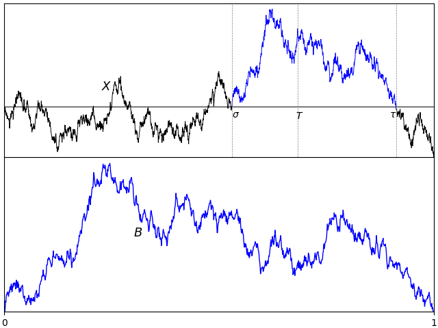
![{\{B_t\}_{t\in[0,T]}}](https://s0.wp.com/latex.php?latex=%7B%5C%7BB_t%5C%7D_%7Bt%5Cin%5B0%2CT%5D%7D%7D&bg=ffffff&fg=000000&s=0&c=20201002) is a Brownian bridge on the interval
is a Brownian bridge on the interval  for a standard Brownian motion X.
 , then B is called a standard Brownian bridge.
  . See lemma
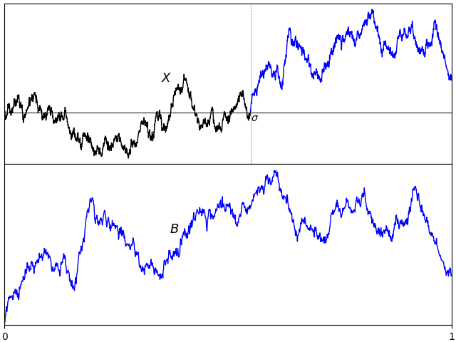
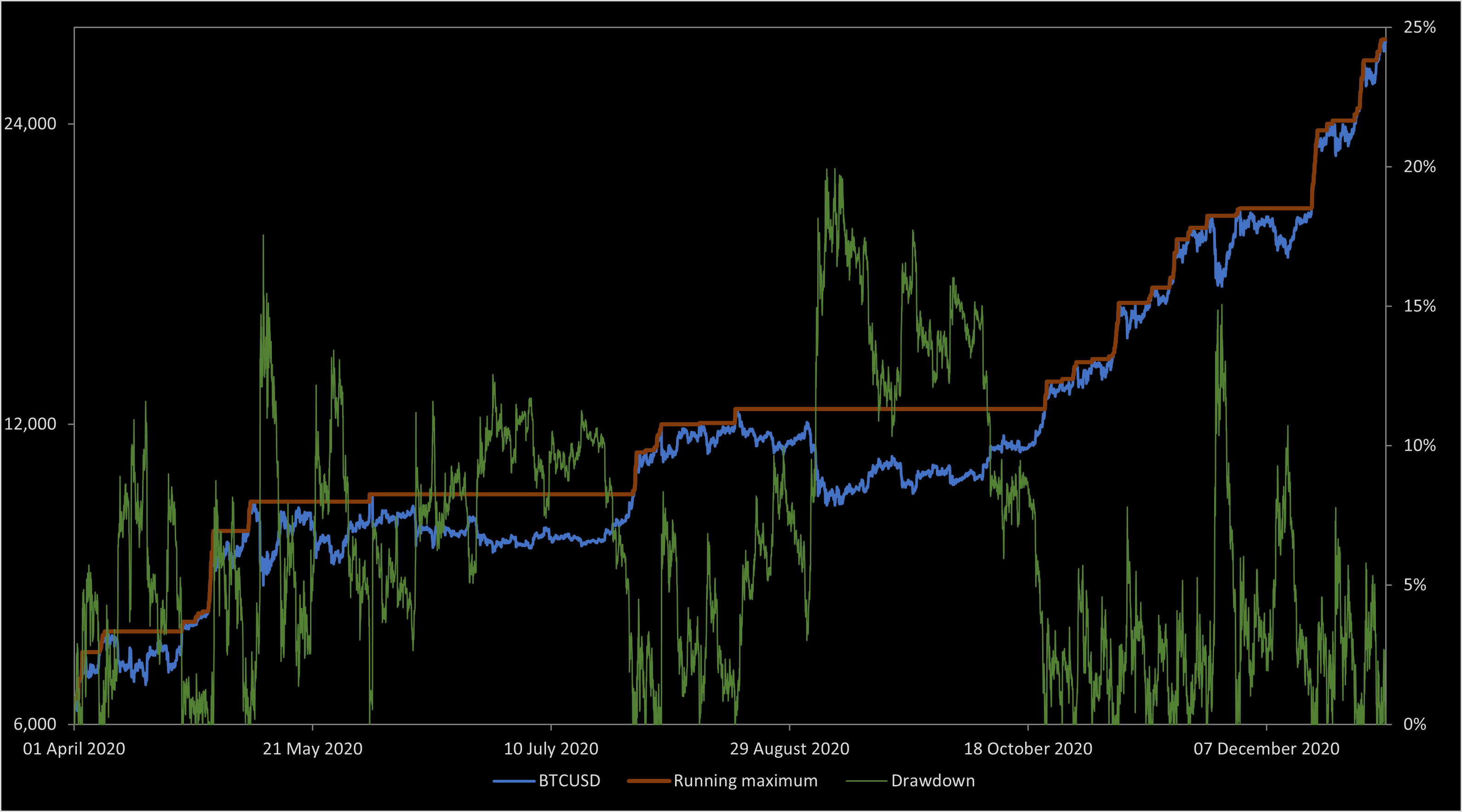
 and drawdown process
  . This is as in figure 1 above.
 was defined to be the drawdown ‘excursion’ over the interval at which the maximum process is equal to the value
  . Precisely, if we let
  be the first time at which X hits level
  and
and  be its right limit
  then,
then,


 , of a Brownian motion, is identical to the distribution of its absolute value and local time at zero,
  . Hence, the point process consisting of the drawdown excursions indexed by the running maximum, and the absolute value of the excursions from zero indexed by the local time, both have the same distribution. So, the theory described in this post applies equally to the excursions away from zero of a Brownian motion.
 , on which we define a canonical process Z by sampling the path at each time t,
  . This space is given the topology of uniform convergence over finite time intervals (compact open topology), which makes it into a Polish space, and whose Borel sigma-algebra
  is equal to the sigma-algebra generated by
  . As shown in the previous post, the counting measure
  is a random point process on
  . In fact, it is a
  .
. is Poisson with intensity measure
  where,
  is the standard Lebesgue measure on
  .
.  is a sigma-finite measure on E given by
![\displaystyle \nu(f) = \lim_{\epsilon\rightarrow0}\epsilon^{-1}{\mathbb E}_\epsilon[f(Z^{\sigma})]](https://s0.wp.com/latex.php?latex=%5Cdisplaystyle++%5Cnu%28f%29+%3D+%5Clim_%7B%5Cepsilon%5Crightarrow0%7D%5Cepsilon%5E%7B-1%7D%7B%5Cmathbb+E%7D_%5Cepsilon%5Bf%28Z%5E%7B%5Csigma%7D%29%5D+&bg=ffffff&fg=000000&s=0&c=20201002)
 which vanish on paths of length less than L (some
  ). The limit is taken over
  ,
,  denotes expectation under the measure with respect to which Z is a Brownian motion started at
  , and
, and  is the first time at which Z hits 0. This measure satisfies the following properties,
  on
on  and
and  everywhere else.
  , the distribution of
  has density
 .
. 
 with running maximum
 from the point process. At least, this can be done so long as the original process does not monotonically increase over any nontrivial intervals, so that there are no intervals with zero drawdown. As the point process indexes the drawdown by the running maximum, we can also reconstruct X as
  . The drawdown point process therefore gives an alternative description of our original process.
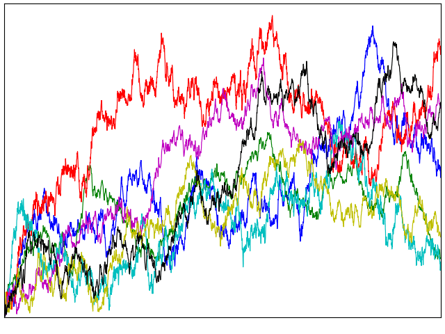
 . It can be noted that, as the price was mostly increasing, the drawdown consists of a relatively large number of small excursions. If, on the other hand, it had declined, then it would have been dominated by a single large drawdown excursion covering most of the time period.
 and that
  tends to infinity as t goes to infinity. Then, for each
  , define the random time at which the process first hits level
 . Each of the excursions on which the drawdown is positive is equal to one of the intervals
  . The excursion is defined as a continuous stochastic process
  equal to the drawdown starting at time
 . Note that there uncountably many values for
  . We will only be interested in these nonzero excursions.
 , so that we have one path of the stochastic process X defined for each
  . Associated to this is the collection of drawdown excursions indexed by the running maximum.
 , which I denote by E. For each time
  , I use
 , so that
  is the measurable space in which the excursion paths lie. It can be seen that
  ,
, 
 .
.  is a measurable random variable for each
  and that there exists a sequence
  covering E such that
  are almost surely finite. The set of drawdowns for the point process corresponding to the bitcoin prices in figure 1 are shown in figure 2 below.
 are disjoint, then the sizes of
  and
and  are independent random variables,
 for each
  ,
, . This justifies the use of Poisson point processes in many different areas of probability and stochastic calculus, and provides a convenient method of showing that point processes are indeed Poisson. If the theorem applies, so that we have a Poisson point process, then we just need to compute the intensity measure to fully determine its distribution. The result above was mentioned in the previous post, but I give a precise statement and proof here.
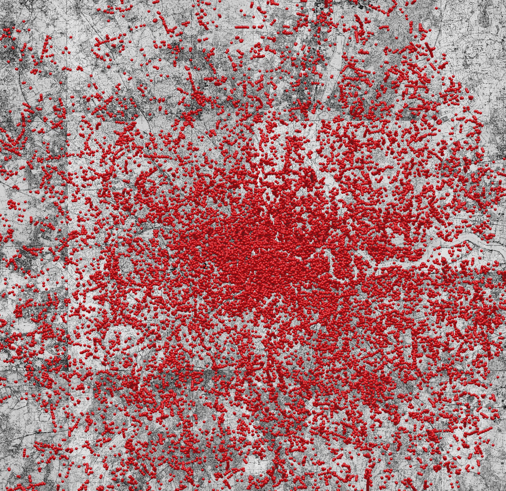
 where, now, F represents the 2-dimensional map and E is used to record both time and location of the bombs. A Poisson point process is a random set of points in E, such that the number that lie within any measurable subset is Poisson distributed. The aim of this post is to introduce Poisson point processes together with the mathematical machinery to handle such random sets.
 are pairwise-disjoint measurable subsets of E, then the sizes of
  are independent.
 -valued stochastic process with independent increments, and which is continuous in probability. Then, the set of points
  over times t for which the jump
  is nonzero gives a Poisson point process on
  . See lemma