
Having previously looked at Brownian bridges and excursions, I now turn to a third kind of process which can be constructed either as a conditioned Brownian motion or by extracting a segment from Brownian motion sample paths. Specifically, the Brownian meander, which is a Brownian motion conditioned to be positive over a unit time interval. Since this requires conditioning on a zero probability event, care must be taken. Instead, it is cleaner to start with an alternative definition by appropriately scaling a segment of a Brownian motion.
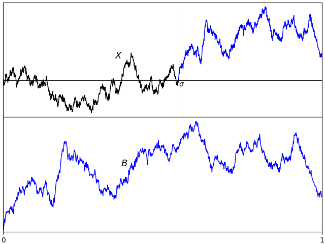
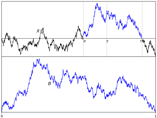
For a fixed positive times T, consider the last time σ before T at which a Brownian motion X is equal to zero,
 |
(1) |
On interval [σ, T], the path of X will start from 0 and then be either strictly positive or strictly negative, and we may as well restrict to the positive case by taking absolute values. Scaling invariance says that c-1/2Xct is itself a standard Brownian motion for any positive constant c. So, scaling the path of X on [σ, 1] to the unit interval defines a process
 |
(2) |
over 0 ≤ t ≤ 1; This starts from zero and is strictly positive at all other times.
Scaling invariance shows that the law of the process B does not depend on the choice of fixed time T The only remaining ambiguity is in the choice of the fixed time T.
Lemma 1 The distribution of B defined by (2) does not depend on the choice of the time T > 0.
Proof: Consider any other fixed positive time T̃, and use the construction above with T̃, σ̃, B̃ in place of T, σ, B respectively. We need to show that B̃ and B have the same distribution. Using the scaling factor S = T̃/T, then X′t = S-1/2XtS is a standard Brownian motion. Also, σ′= σ̃/S is the last time before T at which X′ is zero. So,
 |
has the same distribution as B. ⬜
This leads to the definition used here for Brownian meanders.
Definition 2 A continuous process {Bt}t ∈ [0, 1] is a Brownian meander if and only it has the same distribution as (2) for a standard Brownian motion X and fixed time T > 0.
In fact, there are various alternative — but equivalent — ways in which Brownian excursions can be defined and constructed.
- As a scaled segment of a Brownian motion before a time T and after it last hits 0. This is definition 2.
- As a Brownian motion conditioned on being positive. See theorem 4 below.
- As a segment of a Brownian excursion. See lemma 5.
- As the path of a standard Brownian motion starting from its minimum, in either the forwards or backwards direction. See theorem 6.
- As a Markov process with specified transition probabilities. See theorem 9 below.
- As a solution to an SDE. See theorem 12 below.


![{[0,T]}](https://s0.wp.com/latex.php?latex=%7B%5B0%2CT%5D%7D&bg=ffffff&fg=000000&s=0&c=20201002) is continuous and equal to zero at both endpoints, we can consider extending to the entire real line by partitioning the real numbers into intervals of length T and replicating the path of the process across each of these. This will result in continuous and periodic sample paths, suggesting another method of representing Brownian bridges. That is, by Fourier expansion. As we will see, the Fourier coefficients turn out to be independent normal random variables, giving a useful alternative method of constructing a Brownian bridge.
is continuous and equal to zero at both endpoints, we can consider extending to the entire real line by partitioning the real numbers into intervals of length T and replicating the path of the process across each of these. This will result in continuous and periodic sample paths, suggesting another method of representing Brownian bridges. That is, by Fourier expansion. As we will see, the Fourier coefficients turn out to be independent normal random variables, giving a useful alternative method of constructing a Brownian bridge.![{[0,1]}](https://s0.wp.com/latex.php?latex=%7B%5B0%2C1%5D%7D&bg=ffffff&fg=000000&s=0&c=20201002) . This does not reduce the generality, since bridges on an interval
. This does not reduce the generality, since bridges on an interval 
 , where
  is an IID sequence of standard normals. This series converges uniformly in t, both with probability one and in the
  norm for all
  .
. 
 be a fixed time. Then, the process
 is independent from
  .
.  , we just need to show that
 ![{{\mathbb E}[B_sX_t]}](https://s0.wp.com/latex.php?latex=%7B%7B%5Cmathbb+E%7D%5BB_sX_t%5D%7D&bg=ffffff&fg=000000&s=0&c=20201002) is zero. Using the covariance structure
is zero. Using the covariance structure ![{{\mathbb E}[X_sX_t]=s\wedge t}](https://s0.wp.com/latex.php?latex=%7B%7B%5Cmathbb+E%7D%5BX_sX_t%5D%3Ds%5Cwedge+t%7D&bg=ffffff&fg=000000&s=0&c=20201002) we obtain,
we obtain,![\displaystyle {\mathbb E}[B_sX_t]={\mathbb E}[X_sX_t]-\frac sT{\mathbb E}[X_TX_t]=s-\frac sTT=0](https://s0.wp.com/latex.php?latex=%5Cdisplaystyle++%7B%5Cmathbb+E%7D%5BB_sX_t%5D%3D%7B%5Cmathbb+E%7D%5BX_sX_t%5D-%5Cfrac+sT%7B%5Cmathbb+E%7D%5BX_TX_t%5D%3Ds-%5Cfrac+sTT%3D0+&bg=ffffff&fg=000000&s=0&c=20201002)
![{\{B_t\}_{t\in[0,T]}}](https://s0.wp.com/latex.php?latex=%7B%5C%7BB_t%5C%7D_%7Bt%5Cin%5B0%2CT%5D%7D%7D&bg=ffffff&fg=000000&s=0&c=20201002) is a Brownian bridge on the interval
is a Brownian bridge on the interval  for a standard Brownian motion X.
 , then B is called a standard Brownian bridge.
  . See lemma
 ![\displaystyle \setlength\arraycolsep{2pt} \begin{array}{rl} &\displaystyle{\mathbb E}\left[e^{ia\cdot (X_t-X_0)}\right] = \exp(t\psi(a)),\smallskip\\ &\displaystyle\psi(a)=ia\cdot b-\frac12a^{\rm T}\Sigma a+\int_{{\mathbb R}^d}\left(e^{ia\cdot x}-1-\frac{ia\cdot x}{1+\Vert x\Vert}\right)\,d\nu(x). \end{array}](https://s0.wp.com/latex.php?latex=%5Cdisplaystyle++%5Csetlength%5Carraycolsep%7B2pt%7D+%5Cbegin%7Barray%7D%7Brl%7D+%26%5Cdisplaystyle%7B%5Cmathbb+E%7D%5Cleft%5Be%5E%7Bia%5Ccdot+%28X_t-X_0%29%7D%5Cright%5D+%3D+%5Cexp%28t%5Cpsi%28a%29%29%2C%5Csmallskip%5C%5C+%26%5Cdisplaystyle%5Cpsi%28a%29%3Dia%5Ccdot+b-%5Cfrac12a%5E%7B%5Crm+T%7D%5CSigma+a%2B%5Cint_%7B%7B%5Cmathbb+R%7D%5Ed%7D%5Cleft%28e%5E%7Bia%5Ccdot+x%7D-1-%5Cfrac%7Bia%5Ccdot+x%7D%7B1%2B%5CVert+x%5CVert%7D%5Cright%29%5C%2Cd%5Cnu%28x%29.+%5Cend%7Barray%7D+&bg=ffffff&fg=000000&s=0&c=20201002)

 such that
  is independent of
  for any
  .
.  has the same distribution as
  for any
  .
.  in probability as s tends to t.
 . In that case, we also require that X is adapted to the filtration and that
  for all
  . In particular, if X is a Lévy process according to definition
  . Note that slightly different definitions are sometimes used by different authors. It is often required that
  is zero and that X has
  independently of
  has probability density function p and characteristic function
  given by,
 ![\displaystyle \setlength\arraycolsep{2pt} \begin{array}{rl} &\displaystyle p(x)=\frac{\gamma}{\pi(\gamma^2+x^2)},\smallskip\\ &\displaystyle\phi(a)\equiv{\mathbb E}\left[e^{iaX}\right]=e^{-\gamma\vert a\vert}. \end{array}](https://s0.wp.com/latex.php?latex=%5Cdisplaystyle++%5Csetlength%5Carraycolsep%7B2pt%7D+%5Cbegin%7Barray%7D%7Brl%7D+%26%5Cdisplaystyle+p%28x%29%3D%5Cfrac%7B%5Cgamma%7D%7B%5Cpi%28%5Cgamma%5E2%2Bx%5E2%29%7D%2C%5Csmallskip%5C%5C+%26%5Cdisplaystyle%5Cphi%28a%29%5Cequiv%7B%5Cmathbb+E%7D%5Cleft%5Be%5E%7BiaX%7D%5Cright%5D%3De%5E%7B-%5Cgamma%5Cvert+a%5Cvert%7D.+%5Cend%7Barray%7D+&bg=ffffff&fg=000000&s=0&c=20201002)
 and
and  respectively then
  is Cauchy with parameter
  . We can therefore consistently define a stochastic process
  such that
  , for any
  , where
  describes the covariance structure of the Brownian motion component, b is the drift component, and
  describes the rate at which jumps occur. The distribution of the process is given by the Lévy-Khintchine formula, equation (
 such that
 ![\displaystyle {\mathbb E}\left[e^{ia\cdot (X_t-X_0)}\right]=e^{t\psi(a)}](https://s0.wp.com/latex.php?latex=%5Cdisplaystyle++%7B%5Cmathbb+E%7D%5Cleft%5Be%5E%7Bia%5Ccdot+%28X_t-X_0%29%7D%5Cright%5D%3De%5E%7Bt%5Cpsi%28a%29%7D+&bg=ffffff&fg=000000&s=0&c=20201002)
 and
and  . Also,
  can be written as
 is a positive semidefinite matrix.
  .
.  and,
and,
 .
. has the independent increments property if
  . More generally, we say that X has the independent increments property with respect to an underlying
  where
where  is a measure describing the jumps of X,
  ,
,  such that
  and
and ![\displaystyle {\mathbb E}\left[e^{ia\cdot (X_t-X_0)}\right]=e^{i\psi_t(a)}](https://s0.wp.com/latex.php?latex=%5Cdisplaystyle++%7B%5Cmathbb+E%7D%5Cleft%5Be%5E%7Bia%5Ccdot+%28X_t-X_0%29%7D%5Cright%5D%3De%5E%7Bi%5Cpsi_t%28a%29%7D+&bg=ffffff&fg=000000&s=0&c=20201002)
 can be written as
 ![\displaystyle \psi_t(a)=ia\cdot b_t-\frac{1}{2}a^{\rm T}\Sigma_t a+\int _{{\mathbb R}^d\times[0,t]}\left(e^{ia\cdot x}-1-\frac{ia\cdot x}{1+\Vert x\Vert}\right)\,d\mu(x,s)](https://s0.wp.com/latex.php?latex=%5Cdisplaystyle++%5Cpsi_t%28a%29%3Dia%5Ccdot+b_t-%5Cfrac%7B1%7D%7B2%7Da%5E%7B%5Crm+T%7D%5CSigma_t+a%2B%5Cint+_%7B%7B%5Cmathbb+R%7D%5Ed%5Ctimes%5B0%2Ct%5D%7D%5Cleft%28e%5E%7Bia%5Ccdot+x%7D-1-%5Cfrac%7Bia%5Ccdot+x%7D%7B1%2B%5CVert+x%5CVert%7D%5Cright%29%5C%2Cd%5Cmu%28x%2Cs%29+&bg=ffffff&fg=000000&s=0&c=20201002)
 ,
,  and
and  is a continuous function from
  to
to  such that
  and
and  is positive semidefinite for all
  .
.  is a continuous function from
  .
.  with
with  ,
,  for all
  and,
and,![\displaystyle \int_{{\mathbb R}^d\times[0,t]}\Vert x\Vert^2\wedge 1\,d\mu(x,s)<\infty.](https://s0.wp.com/latex.php?latex=%5Cdisplaystyle++%5Cint_%7B%7B%5Cmathbb+R%7D%5Ed%5Ctimes%5B0%2Ct%5D%7D%5CVert+x%5CVert%5E2%5Cwedge+1%5C%2Cd%5Cmu%28x%2Cs%29%3C%5Cinfty.+&bg=ffffff&fg=000000&s=0&c=20201002)
 has the standard
  are independent normal with zero mean and unit variance. A well known fact of such distributions is that they are invariant under rotations, which has the following consequence. The distribution of
  is invariant under rotations of
  and, hence, is fully determined by the values of
  and
and  . This is known as the
  . The moment generating function can be computed,
![\displaystyle M_Z(\lambda)\equiv{\mathbb E}\left[e^{\lambda Z}\right]=\left(1-2\lambda\right)^{-\frac{n}{2}}\exp\left(\frac{\lambda\mu}{1-2\lambda}\right),](https://s0.wp.com/latex.php?latex=%5Cdisplaystyle++M_Z%28%5Clambda%29%5Cequiv%7B%5Cmathbb+E%7D%5Cleft%5Be%5E%7B%5Clambda+Z%7D%5Cright%5D%3D%5Cleft%281-2%5Clambda%5Cright%29%5E%7B-%5Cfrac%7Bn%7D%7B2%7D%7D%5Cexp%5Cleft%28%5Cfrac%7B%5Clambda%5Cmu%7D%7B1-2%5Clambda%7D%5Cright%29%2C+&bg=ffffff&fg=000000&s=0&c=20201002)
 with real part bounded above by 1/2.
 of an n-dimensional
  be its
  has the following property. For times
  is distributed as
  . This is known as the `n-dimensional’ squared Bessel process, and denoted by
  .
.
![\displaystyle dX = 2\sum_iB^i\,dB^i+\sum_id[B^i].](https://s0.wp.com/latex.php?latex=%5Cdisplaystyle++dX+%3D+2%5Csum_iB%5Ei%5C%2CdB%5Ei%2B%5Csum_id%5BB%5Ei%5D.+&bg=ffffff&fg=000000&s=0&c=20201002)
![{[B^i]_t=t}](https://s0.wp.com/latex.php?latex=%7B%5BB%5Ei%5D_t%3Dt%7D&bg=ffffff&fg=000000&s=0&c=20201002) , the final term on the right-hand-side is equal to
, the final term on the right-hand-side is equal to  . Also, the covarations
 ![{[B^i,B^j]}](https://s0.wp.com/latex.php?latex=%7B%5BB%5Ei%2CB%5Ej%5D%7D&bg=ffffff&fg=000000&s=0&c=20201002) are zero for
are zero for  from which it can be seen that
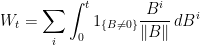
![{[W]_t=t}](https://s0.wp.com/latex.php?latex=%7B%5BW%5D_t%3Dt%7D&bg=ffffff&fg=000000&s=0&c=20201002) . By
. By 
 is not Lipschitz continuous. It is known that (
 . This can be done either by specifying its distributions in terms of chi-square distributions or by the SDE (
 and
and  are independent, then
  has moment generating function
  and, therefore, has the
  distribution. That such distributions do indeed exist can be seen by constructing them. The
  distribution is a special case of the
  . If
. If  , then
  , which can be seen by computing its moment generating function. Adding an independent
  .
. distribution.
  satisfies certain continuity conditions. Many of the standard processes we study satisfy the Feller property, such as
  .
.
 . Equivalently,
 ![\displaystyle {\mathbb E}[f(X_t)\mid\mathcal{F}_s]=P_{t-s}f(X_s)](https://s0.wp.com/latex.php?latex=%5Cdisplaystyle++%7B%5Cmathbb+E%7D%5Bf%28X_t%29%5Cmid%5Cmathcal%7BF%7D_s%5D%3DP_%7Bt-s%7Df%28X_s%29+&bg=ffffff&fg=000000&s=0&c=20201002)
 . The strong Markov property generalizes this idea to arbitrary stopping times.
 be a transition function.
 , conditioned on
  the process
  is Markov with the given transition function and with respect to the filtration
  .
.  . The reflection principle
 defined to be equal to B up until time
 . If
. If  then either the process itself ends up above K or it hits K and then drops below this level by time t, in which case
  . So, by the reflection principle,
 . It will be assumed that E is
  , topological manifolds and, indeed, any open or closed subset of another lccb space. Such spaces are always
  denotes the continuous real-valued functions
  , the set
  is compact. Equivalently, its extension to the
  of E given by
  is continuous. The set
 , so it makes sense to talk of transition probabilities and functions on E.
 ,
,  .
.  is continuous with respect to the norm topology on
  .
.
