Brownian Meanders

Having previously looked at Brownian bridges and excursions, I now turn to a third kind of process which can be constructed either as a conditioned Brownian motion or by extracting a segment from Brownian motion sample paths. Specifically, the Brownian meander, which is a Brownian motion conditioned to be positive over a unit time interval. Since this requires conditioning on a zero probability event, care must be taken. Instead, it is cleaner to start with an alternative definition by appropriately scaling a segment of a Brownian motion.

For a fixed positive times T, consider the last time σ before T at which a Brownian motion X is equal to zero,

$\displaystyle \sigma=\sup\left\{t\le T\colon X_t=0\right\}.$

(1)

On interval [σ, T], the path of X will start from 0 and then be either strictly positive or strictly negative, and we may as well restrict to the positive case by taking absolute values. Scaling invariance says that c^-1/2X_ct is itself a standard Brownian motion for any positive constant c. So, scaling the path of X on [σ, 1] to the unit interval defines a process

$\displaystyle B_t=(T-\sigma)^{-1/2}\lvert X_{\sigma+t(T-\sigma)}\rvert.$

(2)

over 0 ≤ t ≤ 1; This starts from zero and is strictly positive at all other times.

Brownian meander construction — Figure 2: Constructing a Brownian meander

Scaling invariance shows that the law of the process B does not depend on the choice of fixed time T The only remaining ambiguity is in the choice of the fixed time T.

Lemma 1 The distribution of B defined by (2) does not depend on the choice of the time T > 0.

Proof: Consider any other fixed positive time T̃, and use the construction above with T̃, σ̃, B̃ in place of T, σ, B respectively. We need to show that B̃ and B have the same distribution. Using the scaling factor S = T̃/T, then X′_t = S^-1/2X_tS is a standard Brownian motion. Also, σ′= σ̃/S is the last time before T at which X′ is zero. So,

$\displaystyle \tilde B_t=(T-\sigma')^{-1/2}\lvert X'_{\sigma'+t(T-\sigma')}\rvert$

has the same distribution as B. ⬜

This leads to the definition used here for Brownian meanders.

Definition 2 A continuous process {B_t}_{t ∈ [0, 1]} is a Brownian meander if and only it has the same distribution as (2) for a standard Brownian motion X and fixed time T > 0.

In fact, there are various alternative — but equivalent — ways in which Brownian excursions can be defined and constructed.

As a scaled segment of a Brownian motion before a time T and after it last hits 0. This is definition 2.
As a Brownian motion conditioned on being positive. See theorem 4 below.
As a segment of a Brownian excursion. See lemma 5.
As the path of a standard Brownian motion starting from its minimum, in either the forwards or backwards direction. See theorem 6.
As a Markov process with specified transition probabilities. See theorem 9 below.
As a solution to an SDE. See theorem 12 below.

Recall that a standard Brownian motion run up until it last hits 0 before time T is a scaled Brownian bridge. By the definition above, the remaining path after it last hits zero is a Brownian meander. This gives a decomposition of the Brownian path into independent components.

Theorem 3 Let X be a standard Brownian motion, T > 0 be a fixed time and σ < T be as defined by (1). Then, the following collections of random variables are all independent of each other,

The scaled path of X after time σ defined by (2), which is a Brownian meander.

The process σ^-1/2X_tσ over 0 ≤ t ≤ 1, which is a Browian bridge.

σ/T, which has the arcsine distribution.

sgn(X_T), which has the Rademacher distribution.

Proof: Lemma 15 of the Brownian bridge post tells us that σ^-1/2X_tσ is a Brownian bridge independently of the remaining path 1_[τ, T]X, so is independent of the remaining random variables listed.

Next, the distribution of standard Brownian motion is unchanged under flipping the sign, X → –X, and this transformation does not affect the meander given by (2) or the times σ but flips the sign of X_T,. So, sgn(X_T) must have the Rademacher distribution independently of the other random variables.

It just remains to show that σ/T has the arcsine distribution,

$\displaystyle {\mathbb P}(\sigma < s)=\frac2\pi\sin^{-1}\sqrt{\frac sT}$

over s ≤ T, independently of the meander B. As the distribution was already computed in lemma 5 of the post on excursions, only independence remains.

Fixing time s < T, let

$\displaystyle \tau = \inf\{t\ge s\colon X_t=0\}$

so that τ ≤ t precisely on the event that σ ≥ s. By the strong Markov property, X_τ + t is a Brownian motion independent of σ and, by scaling invariance, so is

$\displaystyle \tilde X_t =(1-\tau/T)^{-1/2}X_{\tau+t(1-\tau/T)}$

conditioned on σ < T. However, the Brownian meander defined by (2) using X̃ in place of X is equal to B. Hence, conditioned on σ ≥ s, B still has the distribution of a Brownian meander, showing that it is independent of σ. ⬜

Since the original Brownian motion sample path on interval [0, T] can be reconstructed from the components listed, theorem 3 provides an alternative construction of Brownian motion from independent parts.

As mentioned in the introduction, a meander can be constructed as a Brownian motion conditioned to be positive on the unit interval (0, 1]. As this involves conditioning on a zero probability event, we take a sequence of conditional probabilities for which the Brownian motion is restricted to positive sample paths in the limit. There a various ways in which this limit can be done, but I will use an approach similar to the one in theorem 9 of the Brownian excursion post. We only condition on X being positive after a small positive time ϵ which we allow to go to zero. The weak limit with respect to uniform convergence of sample paths is used, in the same way as in the Brownian excursion post.

Theorem 4 Let {X_t}_{t ∈ [0, 1]} be a standard Brownian motion, and ϵ > 0. Then, the distribution of X conditional on inf_{t ∈ [ϵ, 1]}X_t > 0 converges weakly to that of a Brownian meander as ϵ → 0.

Proof: Theorem 3 says that we can write

$\displaystyle X_t=\begin{cases} \sigma^{1/2}Y_{t/\sigma},&{\rm for\ }t\le\sigma,\\ U(1-\sigma)^{1/2}B_{\sigma+t(1-\sigma)},&{\rm for\ }\sigma\le t\le1\\ \end{cases}$

for a Brownian bridge Y, random time σ, Rademacher variable U and Brownian meander B. In particular, X converges uniformly to B as σ → 0. Furthermore, each of these terms is independent.

The event

$\displaystyle S_\epsilon=\left\{\inf_{t\in[\epsilon,1]}X_t > 0\right\}$

is equivalent to σ < ϵ and U = 1. So, conditioned on S_ϵ, as ϵ goes to zero, the distribution of X converges weakly to that of B which, by independence with S_ϵ, is a Brownian meander. ⬜

Recall that the a Brownian excursion is the path of a Brownian motion over the interval on which it is nonzero about a positive time T, rescaled to the unit time interval. By the definition above, the section of the path just before T is a meander. It follows that a Brownian meander can be constructed as a scaled initial section of an excursion. However, truncating the excursion at a fixed time does not work. Instead, we should truncate at a random time which can be shown to be distributed as the square of a uniform random variable.

Lemma 5 Let X be a Brownian excursion and, independently, U be a random variable uniformly distributed on the unit interval. Then B_t = U^-1X_tU² is a Brownian meander.

Proof: Let σ < T be given by (1) and τ > T be the first time after T at which X hits zero. By the theorem 4 of the Brownian excursion post, B_t = (τ - σ)^-1/2|X_{σ + t(τ - σ)}| is a Brownian excursion independently of σ, τ. Then, by definition 2 above,

$\displaystyle (T-\sigma)^{-1/2}\lvert X_{\sigma+t(T-\sigma)}\rvert=U^{-1}B_{tU^2}$

is a Brownian meander, where U² = (T - σ)/(τ - σ) is independent of B. However, we know the distribution of σ, τ from lemma 5 of the Brownian excursion post:

$\displaystyle {\mathbb P}(\sigma < s,\tau > t)=\frac2\pi\sin^2\sqrt{s/t}.$

Differentiating with respect to s and scaling so that it equals 1 when t = T gives conditional probabilities

$\displaystyle {\mathbb P}(\tau > t\vert\sigma=s)=\sqrt{\frac{T-s}{t-s}}.$

For any continuously distributed real random variable Y with cumulative probability function F(y) = ℙ(Y > y), then F(Y) is uniform on the unit interval. Applying this to the cumulative distribution of τ conditioned on σ computed above shows that U is uniform. ⬜

Brownian motion near a minimum

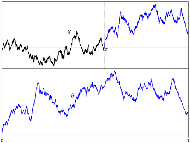
As explained above, for a standard Brownian motion X defined over time interval T, the sample paths after they last hit zero define a Brownian meander. However, there is another method of extracting meanders from the sample paths. Instead of the final time at which it hits zero, consider the time τ^∗ ∈ [0, T] at which X is equal to its pathwise minimum. By definition of the minimum, the section of the sample path started at this time will be bounded below by its initial value and, after subtracting X_τ^∗, will be positive. The same is true for the segment of the path before τ, which we run in reverse time order. After rescaling, this gives a pair of independent meanders.

The idea is as in figure 3 below, where a Brownian motion in the top plot is decomposed into the pair of meanders in the bottom one.

Brownian meander pair — Figure 3: Decomposing a Brownian motion into a pair of meanders

This decomposition is similar in nature to the Vervaat transform from Brownian bridges to excursions. To be precise, I take T = 1 and the two meanders about the minimum of X at time τ are defined by

$\displaystyle \begin{aligned} &Y_t=(1-\tau)^{-1/2}(X_{\tau+t(1-\tau)} - X_\tau),\\ &Z_t=\tau^{-1/2}(X_{(1-t)\tau}-X_\tau), \end{aligned}$

(3)

over 0 ≤ t ≤ 1. The fact that these are independent meanders was shown by Denisov (1984) A Random Walk and a Wiener Process Near a Maximum. Whereas Denisov performs the decomposition about the maximum time, I look at the minimum time here. This is clearly the same thing due to the symmetry of Brownian motion distribution X under reflecting its value about 0. I only use the minimum to avoid reflecting through zero, making the plots in figure 3 a bit easier to visualize. The precise statement which we will prove is:

Theorem 6 Let {X_t}_{t ∈ [0, 1]} be a standard Brownian motion. Then it almost surely has a unique minimum at a time τ, which has the arcsine distribution, and the processes Y, Z are both Brownian meanders. Furthermore, Y, Z and τ are independent.

This result is actually quite intuitive. For any fixed time 0 < τ < 1, then the two processes Y and Z defined by (3) are independent standard Brownian motions. This still holds, if we choose τ randomly and independent of X. Then, conditioning on τ being the time at which X achieves its minimum is the same as conditioning on Y and Z being positive, making them into meanders. However, this idea involves conditioning on zero probability events. It can be made rigorous by taking limits of discrete-time approximations in much the same way as the proof of Vervaat’s transform in the post on excursions.

Instead, I will use a bit of continuous-time stochastic calculus theory to show that the construction of meanders given in figure 3 can be directly translated into the construction (2) used to define Brownian meanders. For a standard Brownian motion X, with running maximum X^∗_t = sup_s ≤ tX_s, then the difference X^∗_t – X_t is a nonnegative process which hits zero every time X reaches a new maximum. This is called the drawdown process of X, as it represents the amount that it has drawn down from its maximum so far. It is well known that this has the same joint distribution as |X_t|, which is a ‘reflecting Brownian motion’. This can be proved by directly showing that X^∗ – X and |X| are both Markov, and computing their transition probabilities. Instead, I will make use of some stochastic integration theory which directly constructs a Brownian motion W for which W^∗ – W = |X|.

As theorem 6 was stated in terms of the minimum instead of the maximum, switch the sign of W so that W – W^m = |X| where W^m_t = inf_s ≤ tW_s is the running minimum. Then, the time τ at which W achieves its minimum value is the same as the final time at which X hits zero, and the process Y defined by (3) (with W in place of X) is exactly the same as the meander B defined by (2). This shows that Y is a Brownian meander by construction, and τ has the arcsine distribution by theorem 3. The process Z is also a Brownian meander by the exact same argument applied to the reversed time Brownian motion W_1 - t – W₁. We still need to show independence, but theorem 6 is almost completed.

Lemma 7 If X is a standard Brownian motion then |X_t|= W_t – W^m_t for standard Brownian motion W defined by

$\displaystyle W_t=\int_0^t1_{\{X_s\not=0\}}d\lvert X_s\rvert.$ (4)

Proof: Using theorem 11 of the post on local times, we have |X|= L + W for standard Brownian motion W and local time L = –W^m which, by lemma 9 of the same post, is given by

$\displaystyle L=\int1_{\{X=0\}}d\lvert X\rvert.$

Plugging this into W = |X|-L and using linearity of expectations gives the result. ⬜

Proving theorem 6 by reducing equations (3) to the construction (2) of a Brownian meander is now almost a formality.

Proof of theorem 6: Starting with standard Brownian motion X, let W be the standard Brownian motion given by lemma 7. If τ is the final time at which W attains its minimum in the unit time interval, then this is the same as the last time at which X is equal to zero. So,

$\displaystyle (1-\tau)^{-1/2}(W_{\tau+t(1-\tau)}-W_\tau)=(1-\tau)^{-1/2}\lvert X_{t+(1-\tau)}\rvert$

which, by construction, is a Brownian meander. Also, theorem 3 shows that this meander, the time τ and the process τ^-1/2X_tτ (over 0 ≤ t ≤ 1) are independent, and τ has the arcsine distribution. As equation (4) expresses W in terms of X, we see that τ^-1/2W_tτ, τ and the meander constructed above are independent. As X and W have the same joint distribution, these statements still hold if W is replaced by X.

So, we have shown that if τ is the last time at which X achieves its minimum then it has the arcsine distribution, the process Y defined by (3) is a Brownian meander, and Y, Z, τ are independent.

Reversing the time direction (replace X_t by X_1 - t – X₁), we see that if τ₀ ≤ τ is the first time at which X hits its minimum over the unit time interval, then this also has the arcsine distribution, so is almost surely equal to τ. It also shows that the process Z defined by (3) is a Brownian meander. ⬜

The Brownian meander distribution

I now explicitly describe the Brownian meander distribution, by showing that it is Markov and computing its transition probabilities. We obtain exact expressions for the probability densities, although they are not as nice as obtained for Brownian bridges or excursions, and does not correspond to any standard distributions which I am aware of. We also do not find constructions of meander sample paths as simple transformations of other standard processes, such as Brownian bridges from Brownian motion and excursions from Bessel processes.

The idea is that, once a Brownian motion becomes positive, it has positive probability of it remaining positive over any given finite time interval. So, it can be directly conditioned on this event. As a meander is just Brownian motion conditioned on being positive, this gives the conditional expectations starting at any positive time.

For real x and t > 0, I use the notation

$\displaystyle \varphi_t(x)=\frac1{\sqrt{2\pi t}}e^{-\frac{x^2}{2t}}$

for the normal density of mean 0 and variance t. I will also write

$\displaystyle \begin{aligned} \Phi_t(x) &=\int_{0}^x\varphi_t(y)\,dy\\ &={\rm erf}(x/\sqrt{2t})/2 \end{aligned}$

(5)

where erf is the error function. For positive x this is the probability of a normally distributed random variable of mean 0 and variance t lying between 0 and x. I will make use of the identity

$\displaystyle {\mathbb E}[{\rm sgn}(U)]=2\Phi_\nu(\mu)$

for a a normal random variable U of mean μ and variance ν. To start, let us consider the distribution of a Brownian motion restricted to being positive over a time interval.

Lemma 8 Let X be a Brownian motion and 0 < t < T be fixed times. Then, conditioned on being positive over the interval [0, T] and on the value of X₀ > 0, the probability density of X_t is

$\displaystyle p_{t,T,X_0}(x)=\left(\varphi_t(x-X_0)-\varphi_t(x+X_0)\right)\Phi_{T-t}(x)/\Phi_T(X_0)$ (6)

over x > 0,.

Proof: Throughout, I will implicitly condition on the value of X₀ > 0, so this can be taken as a fixed positive constant. Letting τ be the first time at which X hits zero, then it is positive over the interval [0, T] if and only if τ > T. For any bounded measurable function f, the reflection principle gives

$\displaystyle {\mathbb E}[f(X_t)1_{\{\tau > T\}}]={\mathbb E}[f(\lvert X_t\rvert){\rm sgn}(X_T)].$

To see this, consider the case where τ ≤ T. Conditioned on this event, the strong Markov property says that X_τ + s is a standard Brownian motion with time index s, so has symmetric distribution under changing its sign. So, it is symmetric under replacing X_T by –X_T. As this also inverts the sign of the expectation on the right hand side above, it must be zero. Hence, the expectation on the right hand side is unchanged if restricted to the event τ > T, giving the left hand side.

As X_T is normal with mean X₀ and variance T, using f = 1 gives

$\displaystyle {\mathbb P}(\tau > T)=2\Phi_T(X_0).$

On the other hand, conditioned on X_t, X_T is normal with mean X_t and variance T – t giving

$\displaystyle \begin{aligned} {\mathbb E}[f(X_t)1_{\{\tau > T\}}] &=2{\mathbb E}\left[f(\lvert X_t\rvert)\Phi_{T-t}(X_t)\right]\\ &=2{\mathbb E}\left[{\rm sgn}(X_t)f(\lvert X_t\rvert)\Phi_{T-t}(\lvert X_t\rvert)\right]. \end{aligned}$

As ±X_t has probability density φ_t(x∓X₀), this shows that restricted to the event τ > T, X_t has density

$\displaystyle \left(\varphi_t(x-X_0)-\varphi_t(x+X_0)\right)\Phi_{T-t}(x)$

over x > 0. To condition on τ > T, we divide through by its probability Φ_T(X₀) to obtain the first expression for p_{t, T, X₀}(x). ⬜

Equation (6) for the transition probabilities can be rearranged as

$\displaystyle \sqrt{\frac2{\pi t}} e^{-\frac1{2t}(x^2+X_0^2)}\sinh\left(\frac{xX_0}t\right)\Phi_{T-t}(x)/\Phi_T(X_0)$

(7)

which can be further simplified to

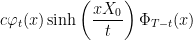$\displaystyle c\varphi_t(x)\sinh\left(\frac{xX_0}t\right)\Phi_{T-t}(x)$

(8)

for a ‘normalizing constant’ c chosen to make this integrate to 1 or, explicitly,

$\displaystyle c=2e^{-\frac{1}{2t}X_0^2}/\Phi_T(X_0).$

Equation (8) can be interpreted as a product of the normalizing constant, the probability density of X_t, the conditional probability of X being positive before t and the conditional probability of it being positive between t and T.

Lemma 8 directly gives the Brownian meander transition probabilities.

Theorem 9 A continuous process {X_t}_{0 ≤ t ≤ 1} is a Brownian meander if and only if it starts from zero and is strictly positive at positive times, and is Markov such that for times 0 < s < t < 1, the distribution of X_t conditioned on X_s has density p_{t - s, 1 - s, X_s} defined by (6).

Proof: Starting with standard Brownian motion X with natural filtration ℱ_·, conditioned on being positive on time interval [ϵ, 1], theorem 4 says that this converges weakly to the law of a Brownian excursion in the limit as ϵ goes to 0.

However, so long as 0 < ϵ < s < t < 1, then conditioned on F_s, X_s + u is a Brownian motion with time index u conditioned to be positive on the inteval [0, 1 - s]. Lemma 8 then says that X_t has probability density p_{t - s, 1 - s, X_s} conditioned on ℱ_s. As this holds for all ϵ < s and is continuous in X_s, it remains true in the limit.

For the converse, it needs to be shown that any positive Markov process with the given transition probabilities and starting from zero is a meander. However, the law of a Markov process is uniquely determined by its initial distribution and transition probabilities. We almost have all of this, but are just missing the transition probabilities for 0 = s < t. These can be computed by taking limit as s and X_s tend to zero, which is the same as computing the distribution of X_t. I do this in Lemma 10 below. ⬜

Since a meander starts from zero, we can take the limit of the transition probabilities as s goes to zero and X_s tends to zero. This gives the probability density of X_t.

Lemma 10 If X is a Brownian meander then X_t has probability density

$\displaystyle 2t^{-3/2}xe^{-\frac{x^2}{2t}}\Phi_{1-t}(x)$

over x > 0, for all 0 < t < 1.

Proof: For time 0 < s < t, theorem 9 says that the probability density of X_t conditional on the value of X_s is p_{t - s, 1 - s, X_s}(x). We just need to take the limit of this as s goes to zero and, by continuity, X_s tends to zero. This is just taking the limit X₀ → 0 in (7) with T = 1. Noting that sinh(xX₀/t) and Φ₁(X₀) both go to zero in this limit, use first order approximations,

$\displaystyle \begin{aligned} \sinh\left(xX_0/t\right)&\sim xX_0/t,\\ \Phi_1(X_0)&\sim X_0/\sqrt{2\pi}, \end{aligned}$

their ratio tends to √2πx/t. Using this in (7) gives the claimed probability density. ⬜

The law of X_t, as described by lemma 10, is not a standard distribution as far as I am aware. At the final time t = 1, however, we obtain the Rayleigh distribution. This is a χ₂ or, equivalently, a square root of the χ²₂ distribution, and also the square root of an exponentially distributed random variable of parameter 1/2. It has probability density xe^–x²/2

Lemma 11 If X is a Brownian meander then X₁ has the Rayleigh distribution.

Proof: The probability density of X₁ can be computed by taking the t → 1 limit in the density described in lemma 10. As the limit of Φ_1 - t(x) is 1/2, we obtain the Rayleigh distribution as claimed. ⬜

The meander SDE

Finally, I look at representing Brownian meanders via a stochastic differential equation (SDE). We should expect this to have a positive drift term which blows up to infinity if the process approaches zero in order to push it away. This is what we saw for the Brownian excursion SDE. In fact, we show that the meander satisfies

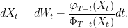$\displaystyle dX_t=dW_t+\frac{\varphi_{T-t}(X_t)}{\Phi_{T-t}(X_t)}dt.$

(9)

for a Brownian motion W. The function Φ_T - t(x), which is defined by (5), vanishes as x goes to zero, so that the drift tends to infinity.

There are several ways in which we can try to prove that SDE (9) is satisfied. First, using the transition probabilities, we could directly show that the difference between X and the drift term is a martingale. This is the approach I used for the Brownian bridge SDE, and would also work here. Second, we could try and express X as a transform of a process whose SDE is already known, such as was done for Brownian excursions although, here, there is no clear way to transform X. The method I will use is Girsanov transforms. By writing X as a Brownian motion under a change of measure, its drift can be computed.

Theorem 12 A continuous process {X_t}_{t ∈ [0, 1]} is a Brownian meander if and only if X₀ = 0 (almost surely) and is strictly positive and solves the SDE (9) over 0 < t ≤ 1 for a standard Brownian motion {W_t}_{t ∈ [0, 1]}.

Proof: Fixing ϵ > 0, it is sufficient to show that the SDE (9) holds over ϵ ≤ t ≤ 1. As previously noted in the proof of theorem 9, on this time range, X has the distribution of a Brownian motion conditioned on being positive. That is, we can suppose that X_t is a Brownian motion over t ≥ ϵ and, letting τ be the first time after ϵ at which it hits zero, we condition on the event {τ > 1}. This conditioning is a continuous change of measure to the new probability distribution ℚ with Radon-Nikodym derivative

$\displaystyle \frac{d{\mathbb Q}}{d{\mathbb P}}\sim 1_{\{\tau > 1\}}.$

I use ∼ to denote that the two sides are equal up to a constant scaling factor (i.e., a normalizing constant to make the total probability equal to 1). As described in the proof of lemma 8, this measure change has conditional expectations

$\displaystyle U_t\equiv{\mathbb E}\left[\frac{d{\mathbb Q}}{d{\mathbb P}}\;\bigg\vert\mathcal F_t\right]\sim1_{\{\tau > t\}}\Phi_{1-t}(X_t).$

for times ϵ ≤ t ≤ 1. Over t < τ this is just Φ_1 - t(X_t) and, as Φ_1 - t(x) has derivative φ_1 - t(x) we compute the quadratic covariation,

$\displaystyle U^{-1}_td[U,X]_t=\frac{\varphi_{1-t}(X_t)}{\Phi_{1-t}(X_t)}dt.$

Theorem 11 of the Girsanov transforms post tells us that, under measure ℚ and for times τ ∧ 1 > t ≥ ϵ, X is a sum of a Brownian motion W and the drift term above. Also, we have τ > 1 almost surely under the measure ℚ, so the result holds over ϵ ≤ t < 1.

Letting ϵ go to zero, this almost completes the proof. There is one slight issue to remaining to address; theorem 11 quoted above is stated for equivalent changes of measure whereas, here, the measure change is only continuous. This is because τ ≤ 1 with positive ℙ-probability, but has zero ℚ-probability. To fix this, choose any δ > 0 and let σ be the first time after ϵ at which X ≤ δ. On the filtration ℱ_σ, the Radon-Nikodym derivative is Φ_1 - σ(X_σ) when σ < 1 and is 1 when σ ≥ 1. As this is strictly positive, the measure change is equivalent on ℱ_σ and, hence, the argument above applies to X up until time σ. Letting δ go to zero, we have σ ≥ 1 eventually, giving the result. ⬜

	Harry on Filtrations and Adapted P…
	Anonymous on Analytic Sets
	Daniel on Analytic Sets
	Sid on Martingale Convergence
	northwiz on Preservation of the Local Mart…
	George Lowther on Martingale Convergence
	Sid on Martingale Convergence
	George Lowther on The Burkholder-Davis-Gundy Ine…
	George Lowther on Preservation of the Local Mart…
	northwiz on Preservation of the Local Mart…