Brownian Motion and the Riemann Zeta Function

Intriguingly, various constructions related to Brownian motion result in quantities with moments described by the Riemann zeta function. These distributions appear in integral representations used to extend the zeta function to the entire complex plane, as described in an earlier post. Now, I look at how they also arise from processes constructed from Brownian motion such as Brownian bridges, excursions and meanders.

Recall the definition of the Riemann zeta function as an infinite series

$\displaystyle \zeta(s)=1+2^{-s}+3^{-s}+4^{-s}+\cdots$

which converges for complex argument s with real part greater than one. This has a unique extension to an analytic function on the complex plane outside of a simple pole at s = 1.

Often, it is more convenient to use the Riemann xi function which can be defined as zeta multiplied by a prefactor involving the gamma function,

$\displaystyle \xi(s)=\frac12s(s-1)\pi^{-s/2}\Gamma(s/2)\zeta(s).$

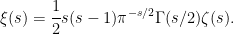
This is an entire function on the complex plane satisfying the functional equation ξ(1 - s) = ξ(s).

It turns out that ξ describes the moments of a probability distribution, according to which a random variable X is positive with moments

$\displaystyle {\mathbb E}[X^s]=2\xi(s),$

(1)

which is well-defined for all complex s. In the post titled The Riemann Zeta Function and Probability Distributions, I denoted this distribution by Ψ, which is a little arbitrary but was the symbol used for its probability density. A related distribution on the positive reals, which we will denote by Φ, is given by the moments

$\displaystyle {\mathbb E}[X^s]=\frac{1-2^{1-s}}{s-1}2\xi(s)$

(2)

which, again, is defined for all complex s.

As standard, complex powers of a positive real x are defined by x^s = e^slogx, so (1,2) are equivalent to the moment generating functions of logX, which uniquely determines the distributions. The probability densities and cumulative distribution functions can be given, although I will not do that here since they are already explicitly written out in the earlier post. I will write X ∼ Φ or X ∼ Ψ to mean that random variable X has the respective distribution. As we previously explained, these are closely connected:

If X ∼ Ψ and, independently, Y is uniform on [1, 2], then X/Y ∼ Φ.
If X, Y ∼ Φ are independent then √X² + Y² ∼ Ψ.

The purpose of this post is to describe some constructions involving Brownian bridges, excursions and meanders which naturally involve the Φ and Ψ distributions.

Theorem 1 The following have distribution Φ:

√2/πZ where Z = sup_t|B_t| is the absolute maximum of a standard Brownian bridge B.

Z/√2π where Z = sup_tB_t is the maximum of a Brownian meander B.

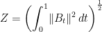
√2πZ where Z is the sample standard deviation of a Brownian bridge B,

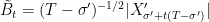
$\displaystyle Z=\left(\int_0^1(B_t-\bar B)^2\,dt\right)^{\frac12}$

with sample mean B̅ = ∫₀¹B_t dt.

√π/2Z where Z is the pathwise Euclidean norm of a 2-dimensional Brownian bridge B = (B¹, B²),

$\displaystyle Z=\left(\int_0^1\lVert B_t\rVert^2\,dt\right)^{\frac12}$

√τπ/2 where τ = inf{t ≥ 0: ‖B_t‖= 1} is the first time at which the norm of a 3-dimensional standard Brownian motion B = (B¹, B², B³) hits 1.

The Kolmogorov distribution is, by definition, the absolute maximum of a Brownian bridge. So, the first statement of theorem 1 is saying that Φ is just the Kolmogorov distribution scaled by the constant factor √2/π. Moving on to Ψ;

Theorem 2 The following have distribution Ψ:

√2/πZ where Z = sup_tB_t – inf_tB_t is the range of a standard Brownian bridge B.

√2/πZ where Z = sup_tB_t is the maximum of a (normalized) Brownian excursion B.

√π/2Z where Z is the pathwise Euclidean norm of a 4-dimensional Brownian bridge B = (B¹, B², B³, B⁴),

$\displaystyle Z=\left(\int_0^1\lVert B_t\rVert^2\,dt\right)^{\frac12}.$

Continue reading “Brownian Motion and the Riemann Zeta Function” →

Brownian Meanders

Having previously looked at Brownian bridges and excursions, I now turn to a third kind of process which can be constructed either as a conditioned Brownian motion or by extracting a segment from Brownian motion sample paths. Specifically, the Brownian meander, which is a Brownian motion conditioned to be positive over a unit time interval. Since this requires conditioning on a zero probability event, care must be taken. Instead, it is cleaner to start with an alternative definition by appropriately scaling a segment of a Brownian motion.

For a fixed positive times T, consider the last time σ before T at which a Brownian motion X is equal to zero,

$\displaystyle \sigma=\sup\left\{t\le T\colon X_t=0\right\}.$

(1)

On interval [σ, T], the path of X will start from 0 and then be either strictly positive or strictly negative, and we may as well restrict to the positive case by taking absolute values. Scaling invariance says that c^-1/2X_ct is itself a standard Brownian motion for any positive constant c. So, scaling the path of X on [σ, 1] to the unit interval defines a process

$\displaystyle B_t=(T-\sigma)^{-1/2}\lvert X_{\sigma+t(T-\sigma)}\rvert.$

(2)

over 0 ≤ t ≤ 1; This starts from zero and is strictly positive at all other times.

Brownian meander construction — Figure 2: Constructing a Brownian meander

Scaling invariance shows that the law of the process B does not depend on the choice of fixed time T The only remaining ambiguity is in the choice of the fixed time T.

Lemma 1 The distribution of B defined by (2) does not depend on the choice of the time T > 0.

Proof: Consider any other fixed positive time T̃, and use the construction above with T̃, σ̃, B̃ in place of T, σ, B respectively. We need to show that B̃ and B have the same distribution. Using the scaling factor S = T̃/T, then X′_t = S^-1/2X_tS is a standard Brownian motion. Also, σ′= σ̃/S is the last time before T at which X′ is zero. So,

$\displaystyle \tilde B_t=(T-\sigma')^{-1/2}\lvert X'_{\sigma'+t(T-\sigma')}\rvert$

has the same distribution as B. ⬜

This leads to the definition used here for Brownian meanders.

Definition 2 A continuous process {B_t}_{t ∈ [0, 1]} is a Brownian meander if and only it has the same distribution as (2) for a standard Brownian motion X and fixed time T > 0.

In fact, there are various alternative — but equivalent — ways in which Brownian excursions can be defined and constructed.

As a scaled segment of a Brownian motion before a time T and after it last hits 0. This is definition 2.
As a Brownian motion conditioned on being positive. See theorem 4 below.
As a segment of a Brownian excursion. See lemma 5.
As the path of a standard Brownian motion starting from its minimum, in either the forwards or backwards direction. See theorem 6.
As a Markov process with specified transition probabilities. See theorem 9 below.
As a solution to an SDE. See theorem 12 below.

Continue reading “Brownian Meanders” →

Brownian Excursions

A normalized Brownian excursion is a nonnegative real-valued process with time ranging over the unit interval, and is equal to zero at the start and end time points. It can be constructed from a standard Brownian motion by conditioning on being nonnegative and equal to zero at the end time. We do have to be careful with this definition, since it involves conditioning on a zero probability event. Alternatively, as the name suggests, Brownian excursions can be understood as the excursions of a Brownian motion X away from zero. By continuity, the set of times at which X is nonzero will be open and, hence, can be written as the union of a collection of disjoint (and stochastic) intervals (σ, τ).

In fact, Brownian motion can be reconstructed by simply joining all of its excursions back together. These are independent processes and identically distributed up to scaling. Because of this, understanding the Brownian excursion process can be very useful in the study of Brownian motion. However, there will by infinitely many excursions over finite time periods, so the procedure of joining them together requires some work. This falls under the umbrella of ‘excursion theory’, which is outside the scope of the current post. Here, I will concentrate on the properties of individual excursions.

In order to select a single interval, start by fixing a time T > 0. As X_T is almost surely nonzero, T will be contained inside one such interval (σ, τ). Explicitly,

$\displaystyle \begin{aligned} &\sigma=\sup\left\{t\le T\colon X_t=0\right\},\\ &\tau=\inf\left\{t\ge T\colon X_t=0\right\}, \end{aligned}$

(1)

so that σ < T < τ < ∞ almost surely. The path of X across such an interval is t ↦ X_σ + t for time t in the range [0, τ - σ]. As it can be either nonnegative or nonpositive, we restrict to the nonnegative case by taking the absolute value. By invariance, S^-1/2X_tS is also a standard Brownian motion, for each fixed S > 0. Using a stochastic factor S = τ – σ, the width of the excursion is normalised to obtain a continuous process {B_t}_{t ∈ [0, 1]} given by

$\displaystyle B_t=(\tau-\sigma)^{-1/2}\lvert X_{\sigma+t(\tau-\sigma)}\rvert.$

(2)

By construction, this is strictly positive over 0 < t < 1 and equal to zero at the endpoints t ∈ {0, 1}.

Figure 2: Constructing a Brownian excursion

The only remaining ambiguity is in the choice of the fixed time T.

Lemma 1 The distribution of B defined by (2) does not depend on the choice of the time T > 0.

Proof: This follows from scaling invariance of Brownian motion. Consider any other fixed positive time T̃, and use the construction above with T̃, σ̃, τ̃, B̃ in place of T, σ, τ, B respectively. We need to show that B̃ and B have the same distribution. Using the scaling factor S = T̃/T, then X′_t = S^-1/2X_tS is a standard Brownian motion. Also, σ′= σ̃/S and τ′= τ̃/S are random times given in the same way as σ and τ, but with the Brownian motion X′ in place of X in (1). So,

$\displaystyle \tilde B_t=(\tau^\prime-\sigma^\prime)^{-1/2}\lvert X^\prime_{\sigma^\prime+t(\tau^\prime-\sigma^\prime)}\rvert$

has the same distribution as B. ⬜

This leads to the definition used here for Brownian excursions.

Definition 2 A continuous process {B_t}_{t ∈ [0, 1]} is a Brownian excursion if and only it has the same distribution as (2) for a standard Brownian motion X and time T > 0.

In fact, there are various alternative — but equivalent — ways in which Brownian excursions can be defined and constructed.

As a normalized excursion away from zero of a Brownian motion. This is definition 2.
As a normalized excursion away from zero of a Brownian bridge. This is theorem 6.
As a Brownian bridge conditioned on being nonnegative. See theorem 9 below.
As the sample path of a Brownian bridge, translated so that it has minimum value zero at time 0. This is a very interesting and useful method of directly computing excursion sample paths from those of a Brownian bridge. See theorem 12 below, sometimes known as the Vervaat transform.
As a Markov process with specified transition probabilities. See theorem 15 below.
As a transformation of Bessel process paths, see theorem 16 below.
As a Bessel bridge of order 3. This can be represented either as a Bessel process conditioned on hitting zero at time 1., or as the vector norm of a 3-dimensional Brownian bridge. See lemma 17 below.
As a solution to a stochastic differential equation. See theorem 18 below.

Continue reading “Brownian Excursions” →

Brownian Drawdowns

BM drawdown — Figure 1: Brownian motion and drawdown

Here, I apply the theory outlined in the previous post to fully describe the drawdown point process of a standard Brownian motion. In fact, as I will show, the drawdowns can all be constructed from independent copies of a single ‘Brownian excursion’ stochastic process. 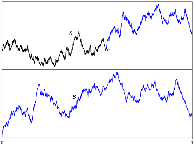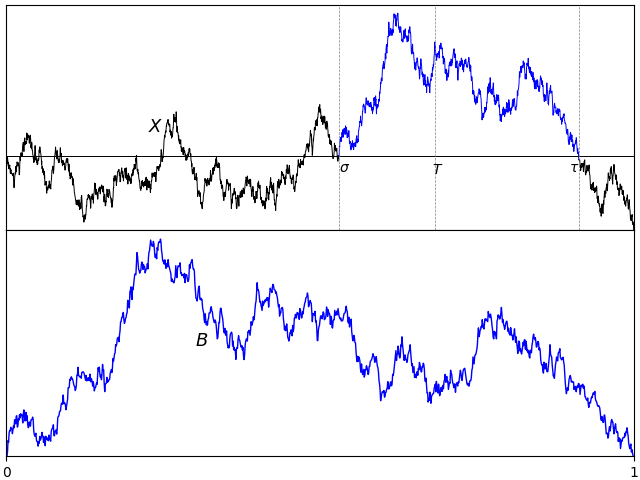Recall that we start with a continuous stochastic process X, assumed here to be Brownian motion, and define its running maximum as ${M_t=\sup_{s\le t}X_s}$ and drawdown process ${D_t=M_t-X_t}$ . This is as in figure 1 above.

Next, ${D^a}$ was defined to be the drawdown ‘excursion’ over the interval at which the maximum process is equal to the value ${a \ge 0}$ . Precisely, if we let ${\tau_a}$ be the first time at which X hits level ${a}$ and ${\tau_{a+}}$ be its right limit ${\tau_{a+}=\lim_{b\downarrow a}\tau_b}$ then,

$\displaystyle D^a_t=D_{({\tau_a+t})\wedge\tau_{a+}}=a-X_{({\tau_a+t)}\wedge\tau_{a+}}.$

Next, a random set S is defined as the collection of all nonzero drawdown excursions indexed the running maximum,

$\displaystyle S=\left\{(a,D^a)\colon D^a\not=0\right\}.$

The set of drawdown excursions corresponding to the sample path from figure 1 are shown in figure 2 below.

BM drawdown excursions — Figure 2: Brownian drawdown excursions

As described in the post on semimartingale local times, the joint distribution of the drawdown and running maximum ${(D,M)}$ , of a Brownian motion, is identical to the distribution of its absolute value and local time at zero, ${(\lvert X\rvert,L^0)}$ . Hence, the point process consisting of the drawdown excursions indexed by the running maximum, and the absolute value of the excursions from zero indexed by the local time, both have the same distribution. So, the theory described in this post applies equally to the excursions away from zero of a Brownian motion.

Before going further, let’s recap some of the technical details. The excursions lie in the space E of continuous paths ${z\colon{\mathbb R}_+\rightarrow{\mathbb R}}$ , on which we define a canonical process Z by sampling the path at each time t, ${Z_t(z)=z_t}$ . This space is given the topology of uniform convergence over finite time intervals (compact open topology), which makes it into a Polish space, and whose Borel sigma-algebra ${\mathcal E}$ is equal to the sigma-algebra generated by ${\{Z_t\}_{t\ge0}}$ . As shown in the previous post, the counting measure ${\xi(A)=\#(S\cap A)}$ is a random point process on ${({\mathbb R}_+\times E,\mathcal B({\mathbb R}_+)\otimes\mathcal E)}$ . In fact, it is a Poisson point process, so its distribution is fully determined by its intensity measure ${\mu={\mathbb E}\xi}$ .

Theorem 1 If X is a standard Brownian motion, then the drawdown point process ${\xi}$ is Poisson with intensity measure ${\mu=\lambda\otimes\nu}$ where,

${\lambda}$ is the standard Lebesgue measure on ${{\mathbb R}_+}$ .

${\nu}$ is a sigma-finite measure on E given by

$\displaystyle \nu(f) = \lim_{\epsilon\rightarrow0}\epsilon^{-1}{\mathbb E}_\epsilon[f(Z^{\sigma})]$ (1)

for all bounded continuous continuous maps ${f\colon E\rightarrow{\mathbb R}}$ which vanish on paths of length less than L (some ${L > 0}$ ). The limit is taken over ${\epsilon > 0}$ , ${{\mathbb E}_\epsilon}$ denotes expectation under the measure with respect to which Z is a Brownian motion started at ${\epsilon}$ , and ${\sigma}$ is the first time at which Z hits 0. This measure satisfies the following properties,

${\nu}$ -almost everywhere, there exists a time ${T > 0}$ such that ${Z > 0}$ on ${(0,T)}$ and ${Z=0}$ everywhere else.

for each ${t > 0}$ , the distribution of ${Z_t}$ has density

$\displaystyle p_t(z)=z\sqrt{\frac 2{\pi t^3}}e^{-\frac{z^2}{2t}}$ (2)

over the range ${z > 0}$ .

over ${t > 0}$ , ${Z_t}$ is Markov, with transition function of a Brownian motion stopped at zero.

Continue reading “Brownian Drawdowns” →

	Harry on Filtrations and Adapted P…
	Anonymous on Analytic Sets
	Daniel on Analytic Sets
	Sid on Martingale Convergence
	northwiz on Preservation of the Local Mart…
	George Lowther on Martingale Convergence
	Sid on Martingale Convergence
	George Lowther on The Burkholder-Davis-Gundy Ine…
	George Lowther on Preservation of the Local Mart…
	northwiz on Preservation of the Local Mart…

Like this:

Like this:

Like this:

Like this: