Brownian Motion and the Riemann Zeta Function

Intriguingly, various constructions related to Brownian motion result in quantities with moments described by the Riemann zeta function. These distributions appear in integral representations used to extend the zeta function to the entire complex plane, as described in an earlier post. Now, I look at how they also arise from processes constructed from Brownian motion such as Brownian bridges, excursions and meanders.

Recall the definition of the Riemann zeta function as an infinite series

$\displaystyle \zeta(s)=1+2^{-s}+3^{-s}+4^{-s}+\cdots$

which converges for complex argument s with real part greater than one. This has a unique extension to an analytic function on the complex plane outside of a simple pole at s = 1.

Often, it is more convenient to use the Riemann xi function which can be defined as zeta multiplied by a prefactor involving the gamma function,

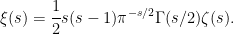$\displaystyle \xi(s)=\frac12s(s-1)\pi^{-s/2}\Gamma(s/2)\zeta(s).$

This is an entire function on the complex plane satisfying the functional equation ξ(1 - s) = ξ(s).

It turns out that ξ describes the moments of a probability distribution, according to which a random variable X is positive with moments

$\displaystyle {\mathbb E}[X^s]=2\xi(s),$

(1)

which is well-defined for all complex s. In the post titled The Riemann Zeta Function and Probability Distributions, I denoted this distribution by Ψ, which is a little arbitrary but was the symbol used for its probability density. A related distribution on the positive reals, which we will denote by Φ, is given by the moments

$\displaystyle {\mathbb E}[X^s]=\frac{1-2^{1-s}}{s-1}2\xi(s)$

(2)

which, again, is defined for all complex s.

As standard, complex powers of a positive real x are defined by x^s = e^slogx, so (1,2) are equivalent to the moment generating functions of logX, which uniquely determines the distributions. The probability densities and cumulative distribution functions can be given, although I will not do that here since they are already explicitly written out in the earlier post. I will write X ∼ Φ or X ∼ Ψ to mean that random variable X has the respective distribution. As we previously explained, these are closely connected:

If X ∼ Ψ and, independently, Y is uniform on [1, 2], then X/Y ∼ Φ.
If X, Y ∼ Φ are independent then √X² + Y² ∼ Ψ.

The purpose of this post is to describe some constructions involving Brownian bridges, excursions and meanders which naturally involve the Φ and Ψ distributions.

Theorem 1 The following have distribution Φ:

√2/πZ where Z = sup_t|B_t| is the absolute maximum of a standard Brownian bridge B.

Z/√2π where Z = sup_tB_t is the maximum of a Brownian meander B.

√2πZ where Z is the sample standard deviation of a Brownian bridge B,

$\displaystyle Z=\left(\int_0^1(B_t-\bar B)^2\,dt\right)^{\frac12}$

with sample mean B̅ = ∫₀¹B_t dt.

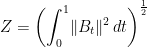
√π/2Z where Z is the pathwise Euclidean norm of a 2-dimensional Brownian bridge B = (B¹, B²),

$\displaystyle Z=\left(\int_0^1\lVert B_t\rVert^2\,dt\right)^{\frac12}$

√τπ/2 where τ = inf{t ≥ 0: ‖B_t‖= 1} is the first time at which the norm of a 3-dimensional standard Brownian motion B = (B¹, B², B³) hits 1.

The Kolmogorov distribution is, by definition, the absolute maximum of a Brownian bridge. So, the first statement of theorem 1 is saying that Φ is just the Kolmogorov distribution scaled by the constant factor √2/π. Moving on to Ψ;

Theorem 2 The following have distribution Ψ:

√2/πZ where Z = sup_tB_t – inf_tB_t is the range of a standard Brownian bridge B.

√2/πZ where Z = sup_tB_t is the maximum of a (normalized) Brownian excursion B.

√π/2Z where Z is the pathwise Euclidean norm of a 4-dimensional Brownian bridge B = (B¹, B², B³, B⁴),

$\displaystyle Z=\left(\int_0^1\lVert B_t\rVert^2\,dt\right)^{\frac12}.$

See the 2001 paper Probability laws related to the Jacobi theta and Riemann zeta functions, and Brownian excursions by Biane, Pitman, and Yor for more information on these and other constructions from stochastic processes resulting in such distributions.

Brownian Bridges

I will start by looking at the various constructions in theorems 1 and 2 involving Brownian bridges. The sample standard deviation described in point 3 of theorem 1 was already proven in lemma 12 of the earlier post, and followed directly from the Fourier expansion of the Brownian bridge. Likewise, statements 4 of theorem 1 and 3 of theorem 2 involving the pathwise Euclidean norms of multidimensional Brownian bridges were proved in theorem 18 of that post.

Moving on to statement 1 of theorem 1, if Z is the absolute maximum of a standard Brownian bridge, we computed its distribution in the post The Minimum and Maximum of Brownian motion. Using corollary 11 from there,

$\displaystyle {\mathbb P}(Z < x)=\frac{\sqrt{2\pi}}{x}\sum_{\substack{n =1\\ n{\rm\ odd}}}^\infty e^{-\frac 12\left(\frac{n\pi}{2x}\right)^2}$

and, if X ∼ Φ, lemma 6 from the earlier post states its distribution function,

$\displaystyle {\mathbb P}(X < x)=2x^{-1}\sum_{n=0}^\infty e^{-\pi(n+1/2)^2x^{-2}}.$

Comparing these shows that √2πZ and X have the same distribution.

This leaves statement 1 of theorem 2 on the range of a Brownian bridge. If we let B^m = inf_tB_t and B^M = sup_tB_t be, respectively, the minimum and maximum, then their joint distribution was computed in theorems 3 and 9 of the post on the minimum and maximum of Brownian motion. Conditioning on X₁ = 0 in those expressions gives the alternative representations,

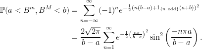$\displaystyle \begin{aligned} {\mathbb P}(a < B^m,B^M < b) &=\sum_{n=-\infty}^\infty(-1)^ne^{-\frac12(n(b-a)+1_{\{n{\rm\ odd}\}}(a+b))^2}\\ &=\frac{2\sqrt{2\pi}}{b-a}\sum_{n=1}^\infty e^{-\frac 12\left(\frac{n\pi}{b-a}\right)^2}\sin^2\left(\frac{-n\pi a}{b-a}\right). \end{aligned}$

These can be transformed to compute the distribution of Z = B^M – B^m.

However, there is a trick. We can use the Vervaat transform described in the post on Brownian excursions. Translating the Brownian bridge so that its minimum value is 0, and translating the time index to start from this minimum, we obtain a Brownian excursion. So, the range of a Brownian bridge is identically distributed to the range of an excursion and, as an excursion has minimum equal to 0, this is identical to the maximum of a Brownian excursion! Hence statement 1 of theorem 2 follows immediately from statement 2, and we do not need to provide an additional proof here.

It is intriguing, though, that if we use the equations above to compute the distribution of Z = B^M – B^m then it gives exactly the same result as I will compute below for the maximum of an excursion. So, I will leave this as an interesting exercise. In fact, historically, the distributions of the range of Brownian bridges and of the maximum of excursions were separately computed and published, and it was noted that they give the result. Only after this, Vervaat published his paper giving the transformation explaining this fact.

Brownian Excursions

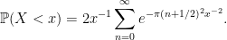
I now look at statement 2 of theorem 2 describing the maximum of a Brownian excursion. If we start with a standard Brownian motion X then, using theorem 9 of the post on the minimum and maximum of Brownian, the joint distribution of its minimum and maximum conditioned on its terminal value is given by,

$\displaystyle \begin{aligned} &{\mathbb P}(a < X_t^m,X_t^M < b\;\vert X_t)\\ &=\frac{2\sqrt{2\pi t}}{b-a}\sum_{n=1}^\infty e^{\frac{X_t^2}{2t}-\frac t2\left(\frac{n\pi}{b-a}\right)^2}\sin\left(\frac{-n\pi a}{b-a}\right)\sin\left(\frac{n\pi(X_t-a)}{b-a}\right) \end{aligned}$

for any a < 0 < b and time t > 0. Only the dependence on b is important so, simplifying,

$\displaystyle \begin{aligned} &{\mathbb P}(X_t^M < b\;\vert X_t=x,a < X_t^m)\\ &=\frac{\kappa}{b-a}\sum_{n=1}^\infty e^{-\frac t2\left(\frac{n\pi}{b-a}\right)^2}\sin\left(\frac{-n\pi a}{b-a}\right)\sin\left(\frac{n\pi(X_t-a)}{b-a}\right) \end{aligned}$

where terms only involving x, a, t have been extracted into the scaling factor κ. Using the approximation sinz ∼ z for small z, we can take limits as t → 1 and a, x → 0 to obtain

$\displaystyle {\mathbb P}(X_t^M < b\;\vert X_t=x,a < X_t^m) \rightarrow\frac{\kappa'}{b^3}\sum_{n=1}^\infty n^2e^{-\frac12n^2\pi^2b^{-2}}$

for a constant κ′. Comparing with the distribution of a random variable Y ∼ Ψ, computed in lemma 6 of the earlier post as,

$\displaystyle {\mathbb P}(Y < b)=\frac{4\pi}{b^3}\sum_{n=1}^\infty n^2e^{-\pi n^2b^{-2}}$

we obtain that X_t^M converges in distribution to √π/2Y.

It just needs to be shown that X_t^M converges in distribution to the maximum of an excursion, and we will be done. In fact, over the range [0, 1], X conditioned on X₁^m > a and X₁ = x will converge weakly to an excursion in the limit as a, x → 0.

This gives what we need, although here I show that it is sufficient to use a simpler result, proven in theorem 9 of the Brownian excursion post. A standard Brownian bridge B conditioned to be positive on time interval [ϵ, 1 - ϵ] tends weakly to an excursion as ϵ → 0. If we set X̃_t = B_ϵ + t – B_ϵ, then this is a Brownian motion conditioned on its final value X̃_1 - 2ϵ = B_1 - ϵ – B_ϵ and, conditioning on B being nonnegative over this range is the same as conditioning on X̃^m_1 - 2ϵ > –B_ϵ. In the limit as ϵ → 0 then –B_ϵ and B_1 - ϵ – B_ϵ tend to zero almost surely. Using what we have just shown above, the maximum of X̃ converges in distribution to √π/2Y but, by theorem 9 of the excursion post, it also converges to the maximum of a Brownian excursion.

This proves statement 2 of theorem 2 and, as discussed above using the Vervaat transform, it also proves statement 1.

Brownian Meanders

Next, I look at point 2 of theorem 1, describing the maximum of a Brownian meander. I will do this now, closely paralleling the proof for the maximum of a Brownian excursion given above.

For a standard Brownian motion X, theorem 7 of the post on the minimum and maximum of Brownian motion states that

$\displaystyle {\mathbb P}\left(a < X_t^m,X_t^M < b\right)=\sum_{\substack{n =1\\ n{\rm\ odd}}}^\infty\frac{4}{n\pi}e^{-\frac t2\left(\frac{n\pi}{b-a}\right)^2}\sin\left(\frac{-n\pi a}{b-a}\right).$

for a < 0 < b. Hence,

$\displaystyle {\mathbb P}\left(X_t^M < b\;\vert a < X_t^m\right)=\kappa\sum_{\substack{n =1\\ n{\rm\ odd}}}^\infty e^{-\frac t2\left(\frac{n\pi}{b-a}\right)^2} n^{-1}\sin\left(\frac{-n\pi a}{b-a}\right)$

for a term κ depending only on a and t. Using the approximation sinz ∼ z as z → 0, we can take the limit as a → 0 and t → 1,

$\displaystyle {\mathbb P}\left(X_t^M < b\;\vert a < X_t^m\right)\rightarrow\kappa'b^{-1}\sum_{\substack{n =1\\ n{\rm\ odd}}}^\infty e^{-\frac 12n^2\pi^2b^{-2}}$

for a constant κ′. Comparing with the distribution of a random variable Y ∼ Φ, computed in lemma 6 of the earlier post as,

$\displaystyle {\mathbb P}(Y < b)=2b^{-1}\sum_{n=0}^\infty e^{-\pi(n+1/2)^2b^{-2}},$

we obtain that X_t^M converges in distribution to √2πY.

It just needs to be shown that X_t^M converges in distribution to the maximum of a meander, and we will be done. In fact, over the range [0, 1], X conditioned on X₁^m > a will converge weakly to a meander in the limit as a → 0.

This gives what we need, although here I show that it is sufficient to use a simpler result, proven in theorem 4 of the Brownian meander post. The standard Brownian motion X conditioned to be positive on time interval [ϵ, 1] tends weakly to a meander as ϵ → 0. If we set X̃_t = X_ϵ + t – X_ϵ, then this is a Brownian motion, and conditioning on X being nonnegative over this range is the same as conditioning on X̃^m_1 - ϵ > –X_ϵ. In the limit as ϵ → 0 then –X_ϵ tends to zero almost surely. Using what we have just shown above, the maximum of X̃ converges in distribution to √2πY but, by theorem 4 of the meander post, it also converges to the maximum of a Brownian meander.

This proves statement 2 of theorem 1 as required.

Stopping Time Distribution

Finally, I look at statement 5 of theorem 1. If B = (B¹, B², B³) is a 3-dimensional standard Brownian motion, then its squared Euclidean norm X = ‖B‖² is a squared Bessel process satisfying the stochastic differential equation

$\displaystyle dX=2\sqrt{X_t}\,dW_t+3dt$

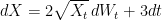for a Brownian motion W. The moment generating function of the first time τ at which it hits 1 can be computed by a general technique for hitting times of diffusions. Choosing constant λ > 0, we will find a continuous function f: ℝ₊ → ℝ such that f(X_t)e^–λt is a local martingale. Once that is done, stopping this at a finite time τ will give a bounded martingale so, by optional sampling,

$\displaystyle {\mathbb E}[f(X_\tau)e^{-\lambda\tau}]=f(0).$

So, as τ is almost surely finite X_τ = 1 by continuity, the moment generating function is given by

$\displaystyle {\mathbb E}[e^{-\lambda\tau}]=f(0)/f(1).$

Let’s compute the function f. Applying Ito’s lemma and substituting in the SDE above for dX,

$\displaystyle \begin{aligned} d\left(f(X_t)e^{-\lambda X_t}\right) =& \left(2X_tf''(X_t)+3f'(X_t)-\lambda f(X_t)\right)e^{-\lambda t}dt\\ &+2f'(X_t)e^{-\lambda t}\sqrt{X_t}\,dW_t. \end{aligned}$

For this to be a local martingale, it is sufficient for the first integral on the right hand side to vanish so that it is an integral with respect to W,

$\displaystyle 2xf''(x)+3f'(x)-\lambda f(x)=0.$

This can be solved by comparing terms in a power series expansion,

$\displaystyle f(x) =\sum_{n=0}^\infty \frac{(2\lambda)^n x^n}{(2n+1)!}=\frac{\sinh\sqrt{2\lambda x}}{\sqrt{2\lambda x}}.$

So, the moment generating function is,

$\displaystyle {\mathbb E}[e^{-\lambda\tau}]=\frac{\sqrt{2\lambda}}{\sinh\sqrt{2\lambda}}.$

Comparing this to the moment generating function of the square of a random variable Z ∼ Φ computed in lemma 8 of the post on the Riemman zeta function and probability distributions,

$\displaystyle {\mathbb E}[e^{-\pi^{-1}\lambda^2Z^2}]=\frac\lambda{\sinh\lambda}$

immediately shows that Z and √τπ/2 are identically distributed.

	Anonymous on About
	Anonymous on About
	Anonymous on The Stochastic Integral
	Anonymous on Bessel Processes
	Anonymous on Bessel Processes
	Stat Prof on Pathwise Regularity of Optiona…
	Yang Chu on Spitzer’s Formula
	Anonymous on About
	Anonymous on Continuous Processes with Inde…
	Anonymous on Continuous Processes with Inde…