A stochastic process X is said to have independent increments if  is independent of
  for all
  . For example, standard Brownian motion is a continuous process with independent increments. Brownian motion also has stationary increments, meaning that the distribution of
  does not depend on t. In fact, as I will show in this post, up to a scaling factor and linear drift term, Brownian motion is the only such process. That is, any continuous real-valued process X with stationary independent increments can be written as
 |
(1) |
for a Brownian motion B and constants  . This is not so surprising in light of the central limit theorem. The increment of a process across an interval [s,t] can be viewed as the sum of its increments over a large number of small time intervals partitioning [s,t]. If these terms are independent with relatively small variance, then the central limit theorem does suggest that their sum should be normally distributed. Together with the previous posts on Lévy’s characterization and stochastic time changes, this provides yet more justification for the ubiquitous position of Brownian motion in the theory of continuous-time processes. Consider, for example, stochastic differential equations such as the Langevin equation. The natural requirements for the stochastic driving term in such equations is that they be continuous with stationary independent increments and, therefore, can be written in terms of Brownian motion.
The definition of standard Brownian motion extends naturally to multidimensional processes and general covariance matrices. A standard d-dimensional Brownian motion  is a continuous process with stationary independent increments such that
  has the
  distribution for all
  . That is, is joint normal with zero mean and covariance matrix tI. From this definition,
  has the
  distribution independently of
  for all . This definition can be further generalized. Given any
  and positive semidefinite
  , we can consider a d-dimensional process X with continuous paths and stationary independent increments such that
  has the
  distribution for all . Here,
  is the drift of the process and
  is the `instantaneous covariance matrix’. Such processes are sometimes referred to as
  -Brownian motions, and all continuous d-dimensional processes starting from zero and with stationary independent increments are of this form.
Theorem 1 Let X be a continuous  -valued process with stationary independent increments.
Then, there exist unique and such that  is a -Brownian motion.
This result is a special case of Theorem 2 below. In particular consider the case of continuous real valued processes with stationary independent increments. Then, by this result, there are constants  such that is normal with mean
  and variance
  for
for  . As long as X is not a deterministic process, so that
  is nonzero,
  will be a standard Brownian motion and (1) is satisfied.
It is also possible to define Gaussian processes with independent but non-stationary increments. Consider continuous functions  and
and  with
with  ,
,  , and such that
  is increasing in the sense that
  is positive semidefinite for all . Then, there will exist processes X with the independent increments property and such that has the
  distribution for all . This exhausts the space of continuous d-dimensional processes with independent incements.
Theorem 2 Let X be a continuous -valued process with the independent increments property.
Then, there exist (unique, continuous) functions and with , such that has the distribution for all  .
.
Note, in particular, that if the increments of X are also stationary, then  and
and  will be independent of t for each fixed
  . It follows that
  and
and  for some
  and
and  . Theorem 1 is then a direct consequence of this result.
Before moving on to the proof of Theorem 2, I should point out that there do indeed exist well-defined processes with the required distributions. First, for the stationary increments case, consider and positive semidefinite . Letting  be the Cholesky decomposition and B be a d-dimensional Brownian motion,
is easily seen to have independent increments with the  distribution. More generally, consider continuous functions and with , and such that is positive semidefinite for . If is absolutely continuous, so that
  for some measurable
  , then X can similarly be expressed in terms of a d-dimensional Brownian motion B. As is increasing,
  will be positive semidefinite for almost all t. Letting
  be its Cholesky decomposition,
 |
(2) |
satisfies the required properties. The  term here is to be interpreted as matrix multiplication,
  . First,
is finite, so  is indeed Bj-integrable. The integral
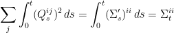
  is also normally distributed with independent increments. If Q is piecewise constant then this follows from the fact that linear combinations of joint normal random variables are normal and the case for general deterministic integrands follows by taking limits. The covariance matrix of can be computed using the Ito isometry,
This identity made use of the covarations ![{[B^i,B^j]_s=\delta_{ij}s}](https://s0.wp.com/latex.php?latex=%7B%5BB%5Ei%2CB%5Ej%5D_s%3D%5Cdelta_%7Bij%7Ds%7D&bg=ffffff&fg=000000&s=0&c=20201002) . So, the process given by (2) does indeed have stationary independent increments with the distribution.
. So, the process given by (2) does indeed have stationary independent increments with the distribution.
Finally, in the general case, a deterministic time change can be applied to force to be absolutely continuous. Define  by
by  . This is continuous and strictly increasing, so has an inverse
  . By positive semidefiniteness
for . So,  is absolutely continuous and, as described above, it is possible to construct a continuous process
  with independent increments from a standard d-dimensional Brownian motion such that
  has the
  distribution for all . Then,
  has the required properties.
Proof of the Theorem
Assume that X is a continuous process with independent increments. If it can be shown that is normal for all , then Theorem 2 will follow by setting
By continuity of X, these are continuous functions. Furthermore, is the covariance matrix of and must be positive semidefinite. In fact it is enough to compute the characteristic function of for all ,
![\displaystyle \setlength\arraycolsep{2pt} \begin{array}{rl} &\displaystyle\phi\colon{\mathbb R}_+\times{\mathbb R}^d\rightarrow{\mathbb C},\smallskip\\ &\displaystyle\phi(t,a)={\mathbb E}\left[e^{ia\cdot(X_t-X_0)}\right]. \end{array}](https://s0.wp.com/latex.php?latex=%5Cdisplaystyle++%5Csetlength%5Carraycolsep%7B2pt%7D+%5Cbegin%7Barray%7D%7Brl%7D+%26%5Cdisplaystyle%5Cphi%5Ccolon%7B%5Cmathbb+R%7D_%2B%5Ctimes%7B%5Cmathbb+R%7D%5Ed%5Crightarrow%7B%5Cmathbb+C%7D%2C%5Csmallskip%5C%5C+%26%5Cdisplaystyle%5Cphi%28t%2Ca%29%3D%7B%5Cmathbb+E%7D%5Cleft%5Be%5E%7Bia%5Ccdot%28X_t-X_0%29%7D%5Cright%5D.+%5Cend%7Barray%7D+&bg=ffffff&fg=000000&s=0&c=20201002) |
(3) |
The characteristic function of can recovered from  by applying the independent increments property,
So, the distribution of is determined by
![\displaystyle {\mathbb E}\left[e^{ia\cdot(X_t-X_s)}\right]=\phi(t,a)/\phi(s,a).](https://s0.wp.com/latex.php?latex=%5Cdisplaystyle++%7B%5Cmathbb+E%7D%5Cleft%5Be%5E%7Bia%5Ccdot%28X_t-X_s%29%7D%5Cright%5D%3D%5Cphi%28t%2Ca%29%2F%5Cphi%28s%2Ca%29.+&bg=ffffff&fg=000000&s=0&c=20201002) |
(4) |
Then, the proof of Theorem 2 requires showing that  has the form of the characteristic function of a normal distribution (for each fixed t). That is, it is the exponential of a quadratic in a.
It is possible to prove the theorem directly, by splitting up into small time increments,
for  . Letting the mesh of this partition go to zero, it is possible to show that only terms up to second order in a contribute to the terms
 ![{{\mathbb E}[e^{ia\cdot(X_{t_k}-X_{t_{k-1}})}]}](https://s0.wp.com/latex.php?latex=%7B%7B%5Cmathbb+E%7D%5Be%5E%7Bia%5Ccdot%28X_%7Bt_k%7D-X_%7Bt_%7Bk-1%7D%7D%29%7D%5D%7D&bg=ffffff&fg=000000&s=0&c=20201002) in the limit. This does involve a tricky argument, taking care to correctly bound the higher order terms.
in the limit. This does involve a tricky argument, taking care to correctly bound the higher order terms.
An alternative approach, which I take here, is to use stochastic calculus. Up to a martingale term, Ito’s lemma enables us to write the logarithm of in terms of X and a quadratic variation term. Then, taking expectations will give the desired quadratic form for  .
.
As always, we will work with respect to a filtered probability space  . In particular, if
  is the natural filtration of a process X with the independent increments property then, for , will be independent of
  . This will be assumed throughout the remainder of this post.
Let us start by showing that the characteristic functions of X have well-defined and continuous logarithms everywhere which, in particular, requires that be everywhere nonzero. On top of the independent increments property, only continuity in probability of X is required. That is,  in probability for all sequences
  of times tending to t. This is a much weaker condition than pathwise continuity.
Lemma 3 Let X be a d-dimensional process which is continuous in probability and has independent increments . Then, there exists a unique continuous function  with
with  and
and
![\displaystyle {\mathbb E}[e^{ia\cdot(X_t-X_0)}]=e^{\psi(t,a)}.](https://s0.wp.com/latex.php?latex=%5Cdisplaystyle++%7B%5Cmathbb+E%7D%5Be%5E%7Bia%5Ccdot%28X_t-X_0%29%7D%5D%3De%5E%7B%5Cpsi%28t%2Ca%29%7D.+&bg=ffffff&fg=000000&s=0&c=20201002) |
(5) |
Furthermore,
 |
(6) |
is a martingale for each fixed  .
.
Proof: First, the function defined by (3) will be continuous. Indeed, if  and
and  then
then  tends to
  in probability and, by bounded convergence,
  . We need to take its logarithm, for which it is necessary to show that it is never zero.
Suppose that  for some t,a. By continuity, for the given value of a, t can be chosen to be minimal. From the definition,
  and t is strictly positive. By the independent increments property, for all
By minimality of t,  is nonzero. Also, by continuity in probability, the second term on the right hand side tends to 1 as s increases to t, so is also nonzero for large enough s. So,
  .
.
We have shown that is a continuous function from  to
to  . It is a standard result from algebraic topology that
  is the covering space of
  with respect to the map
  and, therefore, has a unique lift with
  . That is,
  .
.
More explicitly,  can be constructed as follows. For any positive constants
  , the continuity of implies that there are times
  such that
  for all t in the interval
 ![{[t_k,t_{k+1}]}](https://s0.wp.com/latex.php?latex=%7B%5Bt_k%2Ct_%7Bk%2B1%7D%5D%7D&bg=ffffff&fg=000000&s=0&c=20201002) and
and  . So,
. So,  lies in the right half-plane of . As the complex logarithm is uniquely defined as a continuous function on this region, satisfying
  ,
,  uniquely extends from
  to
to  by
by
So is uniquely defined over  and and, by letting T, K increase to infinity, it is uniquely defined on all of .
It only remains to show that (6) is a martingale, which follows from (4) and the independent increments property,
⬜
Next, we would like to write the characteristic function in terms of the increments
With the aid of Ito’s lemma, it is possible to take logarithms of (6). This shows that, up to a deterministic process, X is a semimartingale, and also gives an expression for up to a martingale term.
Lemma 4 Let X be a continuous d-dimensional process with independent increments and  be as in (5).
Then, there exists a continuous  such that
  is a semimartingale. Furthermore,
![\displaystyle ia\cdot(X_t-X_0)-\psi_t(a)-\frac12[a\cdot\tilde X]_t](https://s0.wp.com/latex.php?latex=%5Cdisplaystyle++ia%5Ccdot%28X_t-X_0%29-%5Cpsi_t%28a%29-%5Cfrac12%5Ba%5Ccdot%5Ctilde+X%5D_t+&bg=ffffff&fg=000000&s=0&c=20201002) |
(7) |
is a square integrable martingale, for all .
The proof of this makes use of complex-valued semimartingales, which are complex valued processes whose real and imaginary parts are both semimartingales. It is easily checked that Ito’s lemma holds for complex semimartingales, simply by applying the result to the real and imaginary parts separately.
Proof: Fixing an , set  . Then, by Lemma 3,
  is a martingale and, hence, a semimartingale. Then, by Ito’s lemma,
  is a semimartingale. Note that, although the logarithm is not a well-defined twice differentiable function everywhere on , this true locally (actually, on any half plane), so there is no problem in applying Ito’s lemma here.
We have shown that  is a semimartingale. Taking imaginary parts,
  is a semimartingale. In particular, writing
  where
where  is the unit vector along the k’th dimension, then
  is a continuous function from
  to and is a semimartingale.
Applying Ito’s lemma again,
As  , U is uniformly bounded over any finite time interval and, in particular, is a square integrable martingale. Similarly,
  is uniformly bounded on any finite time interval, so
![\displaystyle M\equiv\int U^{-1}\,dU = Y+\frac12[Y]](https://s0.wp.com/latex.php?latex=%5Cdisplaystyle++M%5Cequiv%5Cint+U%5E%7B-1%7D%5C%2CdU+%3D+Y%2B%5Cfrac12%5BY%5D+&bg=ffffff&fg=000000&s=0&c=20201002) |
(8) |
is also a square integrable martingale.
Now, Y can be written as  for the process
which is both a semimartingale and a deterministic process. So, the integrals  must be bounded over the set of all piecewise-contant and deterministic processes
  . Therefore, V has bounded variation over each bounded time interval. We have shown that
  plus an FV process, and recalling that continuous FV processes do not contribute to quadratic variations,
Substituting this and the definition of Y back into (8) shows that expression (7) is the square integrable martingale M. ⬜
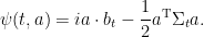
Finally, taking expectations of (7) gives the required form for , showing that is a joint normal random variable for any , and completing the proof of Theorem 2.
Lemma 5 Let X be a continuous d-dimensional process with independent increments, and be as in (5). Then, there are functions and such that
Proof: Taking the imaginary part of (7) shows that  is a martingale. In particular,
  is integrable and, taking expectations,
Taking the real part of (7) shows that ![{\Re\psi_t(a)+\frac12[a\cdot\tilde X]_t}](https://s0.wp.com/latex.php?latex=%7B%5CRe%5Cpsi_t%28a%29%2B%5Cfrac12%5Ba%5Ccdot%5Ctilde+X%5D_t%7D&bg=ffffff&fg=000000&s=0&c=20201002) is a martingale. So,
is a martingale. So, ![{[\tilde X^j,\tilde X^k]}](https://s0.wp.com/latex.php?latex=%7B%5B%5Ctilde+X%5Ej%2C%5Ctilde+X%5Ek%5D%7D&bg=ffffff&fg=000000&s=0&c=20201002) are integrable processes and
are integrable processes and
The result follows by taking ![{b_t={\mathbb E}[X_t-X_0]}](https://s0.wp.com/latex.php?latex=%7Bb_t%3D%7B%5Cmathbb+E%7D%5BX_t-X_0%5D%7D&bg=ffffff&fg=000000&s=0&c=20201002) and
and ![{\Sigma^{jk}_t={\mathbb E}\left[[\tilde X^j,\tilde X^k]_t\right]}](https://s0.wp.com/latex.php?latex=%7B%5CSigma%5E%7Bjk%7D_t%3D%7B%5Cmathbb+E%7D%5Cleft%5B%5B%5Ctilde+X%5Ej%2C%5Ctilde+X%5Ek%5D_t%5Cright%5D%7D&bg=ffffff&fg=000000&s=0&c=20201002) . ⬜
. ⬜


![\displaystyle \setlength\arraycolsep{2pt} \begin{array}{rl} \displaystyle{\mathbb E}\left[(X^i_t-X^i_s)(X^j_t-X^j_s)\right] &\displaystyle={\mathbb E}\left[[X^i,X^j]_t-[X^i,X^j]_s\right]\smallskip\\ &\displaystyle=\sum_{kl}\int_s^tQ^{ik}Q^{jl}\,d[B^k,B^l]\smallskip\\ &\displaystyle=\sum_k\int_s^t Q^{ik}_uQ^{jk}_u\,du=\Sigma^{ij}_t-\Sigma^{ij}_s. \end{array}](https://s0.wp.com/latex.php?latex=%5Cdisplaystyle++%5Csetlength%5Carraycolsep%7B2pt%7D+%5Cbegin%7Barray%7D%7Brl%7D+%5Cdisplaystyle%7B%5Cmathbb+E%7D%5Cleft%5B%28X%5Ei_t-X%5Ei_s%29%28X%5Ej_t-X%5Ej_s%29%5Cright%5D+%26%5Cdisplaystyle%3D%7B%5Cmathbb+E%7D%5Cleft%5B%5BX%5Ei%2CX%5Ej%5D_t-%5BX%5Ei%2CX%5Ej%5D_s%5Cright%5D%5Csmallskip%5C%5C+%26%5Cdisplaystyle%3D%5Csum_%7Bkl%7D%5Cint_s%5EtQ%5E%7Bik%7DQ%5E%7Bjl%7D%5C%2Cd%5BB%5Ek%2CB%5El%5D%5Csmallskip%5C%5C+%26%5Cdisplaystyle%3D%5Csum_k%5Cint_s%5Et+Q%5E%7Bik%7D_uQ%5E%7Bjk%7D_u%5C%2Cdu%3D%5CSigma%5E%7Bij%7D_t-%5CSigma%5E%7Bij%7D_s.+%5Cend%7Barray%7D+&bg=ffffff&fg=000000&s=0&c=20201002)
![\displaystyle b_t={\mathbb E}[X_t-X_0],\ \Sigma_t={\rm Var}(X_t-X_0).](https://s0.wp.com/latex.php?latex=%5Cdisplaystyle++b_t%3D%7B%5Cmathbb+E%7D%5BX_t-X_0%5D%2C%5C+%5CSigma_t%3D%7B%5Crm+Var%7D%28X_t-X_0%29.+&bg=ffffff&fg=000000&s=0&c=20201002)
![\displaystyle {\mathbb E}\left[e^{ia\cdot(X_t-X_0)}\right]= {\mathbb E}\left[e^{ia\cdot(X_t-X_s)}\right] {\mathbb E}\left[e^{ia\cdot(X_s-X_0)}\right].](https://s0.wp.com/latex.php?latex=%5Cdisplaystyle++%7B%5Cmathbb+E%7D%5Cleft%5Be%5E%7Bia%5Ccdot%28X_t-X_0%29%7D%5Cright%5D%3D+%7B%5Cmathbb+E%7D%5Cleft%5Be%5E%7Bia%5Ccdot%28X_t-X_s%29%7D%5Cright%5D+%7B%5Cmathbb+E%7D%5Cleft%5Be%5E%7Bia%5Ccdot%28X_s-X_0%29%7D%5Cright%5D.+&bg=ffffff&fg=000000&s=0&c=20201002)
![\displaystyle \phi(t,a)=\prod_{k=1}^n{\mathbb E}\left[e^{ia\cdot(X_{t_k}-X_{t_{k-1}})}\right]](https://s0.wp.com/latex.php?latex=%5Cdisplaystyle++%5Cphi%28t%2Ca%29%3D%5Cprod_%7Bk%3D1%7D%5En%7B%5Cmathbb+E%7D%5Cleft%5Be%5E%7Bia%5Ccdot%28X_%7Bt_k%7D-X_%7Bt_%7Bk-1%7D%7D%29%7D%5Cright%5D+&bg=ffffff&fg=000000&s=0&c=20201002)
![\displaystyle \phi(t,a)=\phi(s,a){\mathbb E}\left[e^{ia\cdot(X_t-X_s)}\right].](https://s0.wp.com/latex.php?latex=%5Cdisplaystyle++%5Cphi%28t%2Ca%29%3D%5Cphi%28s%2Ca%29%7B%5Cmathbb+E%7D%5Cleft%5Be%5E%7Bia%5Ccdot%28X_t-X_s%29%7D%5Cright%5D.+&bg=ffffff&fg=000000&s=0&c=20201002)

![\displaystyle \setlength\arraycolsep{2pt} \begin{array}{rl} \displaystyle{\mathbb E}\left[e^{ia\cdot X_t-\psi(t,a)}\mid\mathcal{F}_s\right] &\displaystyle=e^{ia\cdot X_s-\psi(t,a)}{\mathbb E}\left[e^{ia\cdot (X_t-X_s)}\mid\mathcal{F}_s\right]\smallskip\\ &\displaystyle=e^{ia\cdot X_s-\psi(t,a)}\phi(t,a)/\phi(s,a)\smallskip\\ &\displaystyle=e^{ia\cdot X_s-\psi(s,a)}. \end{array}](https://s0.wp.com/latex.php?latex=%5Cdisplaystyle++%5Csetlength%5Carraycolsep%7B2pt%7D+%5Cbegin%7Barray%7D%7Brl%7D+%5Cdisplaystyle%7B%5Cmathbb+E%7D%5Cleft%5Be%5E%7Bia%5Ccdot+X_t-%5Cpsi%28t%2Ca%29%7D%5Cmid%5Cmathcal%7BF%7D_s%5Cright%5D+%26%5Cdisplaystyle%3De%5E%7Bia%5Ccdot+X_s-%5Cpsi%28t%2Ca%29%7D%7B%5Cmathbb+E%7D%5Cleft%5Be%5E%7Bia%5Ccdot+%28X_t-X_s%29%7D%5Cmid%5Cmathcal%7BF%7D_s%5Cright%5D%5Csmallskip%5C%5C+%26%5Cdisplaystyle%3De%5E%7Bia%5Ccdot+X_s-%5Cpsi%28t%2Ca%29%7D%5Cphi%28t%2Ca%29%2F%5Cphi%28s%2Ca%29%5Csmallskip%5C%5C+%26%5Cdisplaystyle%3De%5E%7Bia%5Ccdot+X_s-%5Cpsi%28s%2Ca%29%7D.+%5Cend%7Barray%7D+&bg=ffffff&fg=000000&s=0&c=20201002)
![\displaystyle U_t=1+\int_0^tU_s\,dY_s + \frac12\int_0^tU_s\,d[Y]_s.](https://s0.wp.com/latex.php?latex=%5Cdisplaystyle++U_t%3D1%2B%5Cint_0%5EtU_s%5C%2CdY_s+%2B+%5Cfrac12%5Cint_0%5EtU_s%5C%2Cd%5BY%5D_s.+&bg=ffffff&fg=000000&s=0&c=20201002)

![\displaystyle [Y]=[ia\cdot\tilde X]=-[a\cdot\tilde X].](https://s0.wp.com/latex.php?latex=%5Cdisplaystyle++%5BY%5D%3D%5Bia%5Ccdot%5Ctilde+X%5D%3D-%5Ba%5Ccdot%5Ctilde+X%5D.+&bg=ffffff&fg=000000&s=0&c=20201002)
![\displaystyle \Im\psi_t(a)=a\cdot{\mathbb E}[X_t-X_0].](https://s0.wp.com/latex.php?latex=%5Cdisplaystyle++%5CIm%5Cpsi_t%28a%29%3Da%5Ccdot%7B%5Cmathbb+E%7D%5BX_t-X_0%5D.+&bg=ffffff&fg=000000&s=0&c=20201002)
![\displaystyle \Re\psi_t(a)=-\frac12{\mathbb E}\left[[a\cdot\tilde X]_t\right]=-\frac12\sum_{jk}a_ja_k{\mathbb E}\left[[\tilde X^j,\tilde X^k]_t\right].](https://s0.wp.com/latex.php?latex=%5Cdisplaystyle++%5CRe%5Cpsi_t%28a%29%3D-%5Cfrac12%7B%5Cmathbb+E%7D%5Cleft%5B%5Ba%5Ccdot%5Ctilde+X%5D_t%5Cright%5D%3D-%5Cfrac12%5Csum_%7Bjk%7Da_ja_k%7B%5Cmathbb+E%7D%5Cleft%5B%5B%5Ctilde+X%5Ej%2C%5Ctilde+X%5Ek%5D_t%5Cright%5D.+&bg=ffffff&fg=000000&s=0&c=20201002)

Let Y and Z two brownian motions and the process X = pY +(1-p^2)^0.5 Z, where p is between -1 and 1. Assuming X is continuous and has marginal distributions N(0,t). Is X a brownian motion?
Another similar example….if Z is a normal (0,1) the process X(t) = t^0.5 Z is continuous and marginally distributed as a normal N(0,t). But is X a brownian motion?
I am confused how to prove the independent increments property or how to verify it. Any suggestions?
Hi. You don’t need any advanced results to consider the examples you mention. If Y,Z are independent Brownian motions then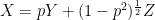 will be a Brownian motion. This just uses the fact that a sum of independent normals is normal, so you can calculate the distribution X. If you aren’t assuming that they are independent then it will depend on precisely what you are assuming, and X does not have to be a Brownian motion in general.
The process is not a Brownian motion, as its increments are all proportional to Z, so are not independent.
Hi, is your definition equivalent to the one commonly used:
For any $n$ and any times $0<s_1<t_1<\ldots < s_n<t_n$, the random variables $\{X_{t_i}-X_{s_i}\}$ are independent?
Hi George, could you explain in a bit more detail how Ito’s lemma applies to log(U) in the proof of Lemma 4?
So U would be the continuous semimartingale and f is the complex logarithm in the original Ito’s lemma. To apply Ito’s lemma we need U to take values in C – some branch cut.
But from the formula of exp(Y), I can only see that it must not take the value 0. So how do we ensure that U will not take values in some branch cut of the complex logarithm?
Hi. You asked quite a few questions. I will answer when I have time, but starting on this one:
As written here, I am using Ito’s formula *locally*. i.e., once you have proved that Y is a semimartingale when stopped at a stopping time tau, you can let tau’ be the first time that Y(tau’)/Y(tau) is imaginary, so we remain in the same half-plane for times tau <= t <= tau'. Hence, the Branch cut can be chosen to miss this half-plane. Apply Ito's formula to the process started at time tau and stopped at tau'.
There are technical details here, but it is just managing the definitions of stopping times, semimartingales, etc. Nothing advanced is really going on.
If you really wanted to get deep in the maths, and formalize these ideas. You could consider semimartingales on a smooth (or C2) manifold, and lift them to the covering space, which is also a C2 manifold. Then, log is defined, and twice differentiable on the covering space of the complex numbers minus the origin.
Thank you George but I am not familiar with this idea. Could you help me understand a bit more? So we want to show that Y=log(U) is a semimartingale knowing that U is a semimartingale.
I can’t see how we can prove that Y is a semimartingale when stopped at any stopping time tau.
I think you mean that U is a semimartingale when stopped at tau? This would be true since U is already a semimartingale and stopping preserves semimartingale. And we can take tau’ as you suggest.
But if U is a semimartingale, is U_\tau also a semimartingale?
And how do we exactly define a process that starts at some stopping time tau and stops at tau’?
Stopping at tau’ can be done by the usual process of U^\tau’. But I don’t know how we can just start it at some stopping time and how that would still preserve the semimartingale property.
Finally, I guess you mean we can then apply Ito’s formula to the process U starting at tau and stopping at tau’ since it would stay in the same half plane. Then we get that log(U)=Y starting at tau and stopping at tau’ is a semimartingale. But how does this prove that Y is a semimartingale? To be a semimartingale or equivalently, locally a semimartingale, we need some sequence tau_n increasing to infinity and Y^\tau_n to be a semimartingale. But the way we define tau’, we cannot guarantee that we can find a sequence increasing to infinity.
Sorry to bother you with details but it is my first time seeing this kind of argument and I haven’t been able to get help elsewhere so I would greatly appreciate your help.
Hello, I was going through the proof and need help with one part. It was mentioned that a (continuous) semimartingale that is deterministic has finite variation (the paragraph after equation 8). I think this seems intuitively correct as the unique martingale component will result in “large local variation with non 0 quadratic variation” but I cant seem to prove it rigirously. Will be glad if you could provide a reference. Thank you!
There are various ways of showing that a process is a semimartingale. Here, I am using the fact that a C2 function of a semimartingale is again a semimartingale, plus additional basic facts (like a semimartingale stopped at a stopping time is a semimartingale).
Anyway, the idea here is define stopping times tau_n inductively by tau_0=0 and tau_{n+1} >= tau_n being the first time at which U_t/U_{tau_n} is imaginary.
We can show that Y=log(U) is a ‘semimartingale on each interval [tau_n,tau_{n+1}]’, since we can choose a branch of log defined and C2 for U_t over this interval.
– But how to interpret the statement that something is a semiartingale on a stochastic interval?
there’s various ways. We can stop it at time tau_{n+1}, and ‘start’ it at tau_n. Either look at the process U_{tau_n+t} with time shifted so that it starts at tau_n. Or, look at Y_t-Y_{tau_n}=log(U_t/U_{tau_n}), but set this to 0 before time tau_n.
Either way works. And, by adding together (or otherwise combining) the processes over each interval, you should be able to show that the stopped processes Y^{tau_n} are semimartingales, implying that Y is a semimartingale.
Makes total sense now thank you for the kind explanation George.
Hello,
I am not sure if I follow the part where it says a deterministic semimartingale has finite variation. (In the paragraph after paragraph 8). Will be grateful if you could provide a reference. Thanks!