
In this post I look at the integral Xt = ∫0t 1{W≥0} dW for standard Brownian motion W. This is a particularly interesting example of stochastic integration with connections to local times, option pricing and hedging, and demonstrates behaviour not seen for deterministic integrals that can seem counter-intuitive. For a start, X is a martingale so has zero expectation. To some it might, at first, seem that X is nonnegative and — furthermore — equals W ∨ 0. However, this has positive expectation contradicting the first property. In fact, X can go negative and we can compute its distribution. In a Twitter post, Oswin So asked about this very point, showing some plots demonstrating the behaviour of the integral.

We can evaluate the integral as Xt = Wt ∨ 0 – 12 Lt0 where Lt0 is the local time of W at 0. The local time is a continuous increasing process starting from 0, and only increases at times where W = 0. That is, it is constant over intervals on which W is nonzero. The first term, Wt ∨ 0 has probability density p(x) equal to that of a normal density over x > 0 and has a delta function at zero. Subtracting the nonnegative value L0t spreads out the density of this delta function to the left, leading to the odd looking density computed numerically in So’s Twitter post, with a peak just to the left of the origin and dropping instantly to a smaller value on the right. We will compute an exact form for this probability density but, first, let’s look at an intuitive interpretation in the language of option pricing.
Consider a financial asset such as a stock, whose spot price at time t is St. We suppose that the price is defined at all times t ≥ 0 and has continuous sample paths. Furthermore, suppose that we can buy and sell at spot any time with no transaction costs. A call option of strike price K and maturity T pays out the cash value (ST - K)+ at time T. For simplicity, assume that this is ‘out of the money’ at the initial time, meaning that S0 ≤ K.
The idea of option hedging is, starting with an initial investment, to trade in the stock in such a way that at maturity T, the value of our trading portfolio is equal to (ST - K)+. This synthetically replicates the option. A naive suggestion which is sometimes considered is to hold one unit of stock at all times t for which St ≥ K and zero units at all other times.The profit from such a strategy is given by the integral XT = ∫0T 1{S≥K} dS. If the stock only equals the strike price at finitely many times then this works. If it first hits K at time s and does not drop back below it on interval (s, t) then the profit at t is equal to the amount St – K that it has gone up since we purchased it. If it drops back below the strike then we sell at K for zero profit or loss, and this repeats for subsequent times that it exceeds K. So, at time T, we hold one unit of stock if its value is above K for a profit of ST – K and zero units for zero profit otherwise. This replicates the option payoff.
The idea described works if ST hits the strike K at a finite set of times,and also if the path of St has finite variation, in which case Lebesgue-Stieltjes integration gives XT = (ST - K)+. It cannot work for stock prices though! If it did, then we have a trading strategy which is guaranteed to never lose money but generates profits on the positive probability event that ST > K. This is arbitrage, generating money with zero risk, which should be impossible.
What goes wrong? First, Brownian motion does not have sample paths with finite variation and will not hit a level finitely often. Instead, if it reaches K then it hits the level uncountably often. As our simple trading strategy would involve buying and selling infinitely often, it is not so easy. Instead, we can approximate by a discrete-time strategy and take the limit. Choosing a finite sequence of times 0 = t0 < t1 < ⋯< tn = T, the discrete approximation is to hold one unit of the asset over the interval (ti, ti+1] if Sti ≥ K and zero units otherwise.
The discrete strategy involves buying one unit of the asset whenever its price reaches K at one of the discrete times and selling whenever it drops back below. This replicates the option payoff, except for the fact then when we buy above K we effectively overpay by amount Sti – K and, when we sell below K, we lose K – Sti. This results in some slippage from not being able to execute at the exact level,
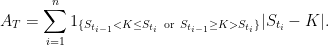 |
So, our simple trading strategy generates profit (ST - K)+ – AT, missing the option value by amount AT. In the limit as n goes to infinity with time step size going to zero, the slippage AT does not go to zero. For equally spaced times, It can be shown that the number of times that spot crosses K is of order √n, and each of these times generates slippage of order 1/√n on average. So, in the limit, AT does not vanish and, instead, converges on a positive value equal to half the local time LTK.

Figure 2 shows the situation, with the slippage A shown on the same plot (using K as the zero axis, so they are on the same scale). We can just take K = 0 for an asset whose spot price can be positive or negative. Then, with S = W, our integral XT = ∫0T 1{W≥0} dW is the same as the payoff from the naive option hedge, or (ST)+ minus slippage L0T/2.
Now lets turn to a computation of the probability density of XT = WT ∨ 0 – LT0/2. By the scaling property of Brownian motion, the distribution of XT/√T does not depend on T, so we take T = 1 without loss of generality. The first trick to this is to make use of the fact that, if Mt = sups≤tWs is the running maximum then (|Wt|, Lt0) has the same joint distribution as (Mt - Wt, Mt). This immediately tells us that L10 has the same distribution as M1 which, by the reflection principle, has the same distribution as |W1|. Using
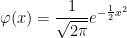 |
for the standard normal density, this shows that the local time L10 has probability density 2φ(x) over x > 0.
Next, as flipping the sign W does not impact either |W1| or L10, sgn(W1) is independent of these. On the event W1 < 0 we have X1 = –L10/2 which has density 4φ(2x) over x < 0. On the event W1 > 0, we have X1 = |W1|-L10/2, which has the same distribution as M1/2 – W1.
To complete the computation of the probability density of X1, we need to know the joint distribution of M1 and W1, which can be done as described in the post on the reflection principle. The probability that W1 is in an interval of width δx about a point x and that M1 > y, for some y > x is, by reflection, equal to the probability that W1 is in an interval of width δx about the point 2y – x. This has probability φ(2y - x)δx and, by differentiating in y, gives a joint probability density of 2φ′(x - 2y) for (W1, M1).
The expectation of f(X1) for bounded measurable function f can be computed by integrating over this joint probability density.
![\displaystyle \begin{aligned} {\mathbb E}[f(X_1)\vert\;W_1 > 0] &={\mathbb E}[f(M_1/2-W_1)]\\ &=2\int_{-\infty}^\infty\int_{x_+}^\infty f(y/2-x)\varphi'(x-2y)\,dydx\\ &=4\int_{-\infty}^\infty\int_{(-x)\vee(-x/2)}^\infty f(z)\varphi'(-3x-4z)\,dzdx\\ &=4\int_{-\infty}^\infty\int_{(-z)\vee(-2z)}^\infty f(z)\varphi'(-3x-4z)\,dxdz\\ &=\frac43\int_{-\infty}^\infty f(z)\varphi(2z)\,dz+\frac43\int_0^\infty f(z)\varphi(z)\,dz. \end{aligned}](https://s0.wp.com/latex.php?latex=%5Cdisplaystyle+%5Cbegin%7Baligned%7D+%7B%5Cmathbb+E%7D%5Bf%28X_1%29%5Cvert%5C%3BW_1+%3E+0%5D+%26%3D%7B%5Cmathbb+E%7D%5Bf%28M_1%2F2-W_1%29%5D%5C%5C+%26%3D2%5Cint_%7B-%5Cinfty%7D%5E%5Cinfty%5Cint_%7Bx_%2B%7D%5E%5Cinfty+f%28y%2F2-x%29%5Cvarphi%27%28x-2y%29%5C%2Cdydx%5C%5C+%26%3D4%5Cint_%7B-%5Cinfty%7D%5E%5Cinfty%5Cint_%7B%28-x%29%5Cvee%28-x%2F2%29%7D%5E%5Cinfty+f%28z%29%5Cvarphi%27%28-3x-4z%29%5C%2Cdzdx%5C%5C+%26%3D4%5Cint_%7B-%5Cinfty%7D%5E%5Cinfty%5Cint_%7B%28-z%29%5Cvee%28-2z%29%7D%5E%5Cinfty+f%28z%29%5Cvarphi%27%28-3x-4z%29%5C%2Cdxdz%5C%5C+%26%3D%5Cfrac43%5Cint_%7B-%5Cinfty%7D%5E%5Cinfty+f%28z%29%5Cvarphi%282z%29%5C%2Cdz%2B%5Cfrac43%5Cint_0%5E%5Cinfty+f%28z%29%5Cvarphi%28z%29%5C%2Cdz.+%5Cend%7Baligned%7D+&bg=ffffff&fg=000000&s=0&c=20201002) |
The substitution z = y/2 – x was applied in the inner integral, and the order of integration switched. The probability density of X1 conditioned on W1 > 0 is therefore,
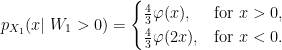 |
Conditioned on W1 < 0, we have already shown that the density is 4φ(2x) over x < 0 so, taking the average of these, we obtain
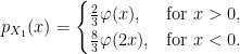 |
This is plotted in figure 3 below, agreeing with So’s numerical estimation from the Twitter post shown in figure 1 above.


![\displaystyle {\mathbb E}[g(X_t)\;\vert\mathcal F_s]=f(X_s,s).](https://s0.wp.com/latex.php?latex=%5Cdisplaystyle+%7B%5Cmathbb+E%7D%5Bg%28X_t%29%5C%3B%5Cvert%5Cmathcal+F_s%5D%3Df%28X_s%2Cs%29.+&bg=ffffff&fg=000000&s=0&c=20201002)


 , a map
  between metric spaces E and F is said to be
 . The smallest value of C satisfying this inequality is known as the
  . Hölder continuous functions are always continuous and, at least on bounded spaces, is a stronger property for larger values of the coefficient
  , then every
  -Hölder continuous map from E is also
  -Hölder continuous. In particular, 1-Hölder and Lipschitz continuity are equivalent.
 are almost surely locally Hölder continuous. That is, they are almost surely Hölder continuous on every bounded interval. To start with, we look at real-valued processes. Throughout this post, we work with repect to a probability space
  . There is no need to assume the existence of any filtration, since they play no part in the results here
 be a real-valued stochastic process such that there exists positive constants
  satisfying
 ![\displaystyle {\mathbb E}\left[\lvert X_t-X_s\rvert^\alpha\right]\le C\lvert t-s\vert^{1+\beta},](https://s0.wp.com/latex.php?latex=%5Cdisplaystyle++%7B%5Cmathbb+E%7D%5Cleft%5B%5Clvert+X_t-X_s%5Crvert%5E%5Calpha%5Cright%5D%5Cle+C%5Clvert+t-s%5Cvert%5E%7B1%2B%5Cbeta%7D%2C+&bg=ffffff&fg=000000&s=0&c=20201002)
 . Then, X has a continuous modification which, with probability one, is locally
  .
. ![\displaystyle c_p^{-1}{\mathbb E}[[M]^{p/2}_\tau]\le{\mathbb E}[\bar M_\tau^p]\le C_p{\mathbb E}[[M]^{p/2}_\tau].](https://s0.wp.com/latex.php?latex=%5Cdisplaystyle++c_p%5E%7B-1%7D%7B%5Cmathbb+E%7D%5B%5BM%5D%5E%7Bp%2F2%7D_%5Ctau%5D%5Cle%7B%5Cmathbb+E%7D%5B%5Cbar+M_%5Ctau%5Ep%5D%5Cle+C_p%7B%5Cmathbb+E%7D%5B%5BM%5D%5E%7Bp%2F2%7D_%5Ctau%5D.+&bg=ffffff&fg=000000&s=0&c=20201002)
 is the running maximum,
 ![{[M]}](https://s0.wp.com/latex.php?latex=%7B%5BM%5D%7D&bg=ffffff&fg=000000&s=0&c=20201002) is the quadratic variation,
is the quadratic variation,  is a
is a  is a real number greater than or equal to 1. Then,
  and
and  are positive constants depending on p, but independent of the choice of local martingale and stopping time. Furthermore, for continuous local martingales, which are the focus of this post, the inequality holds for all
  .
.![{[M]_0=M_0^2}](https://s0.wp.com/latex.php?latex=%7B%5BM%5D_0%3DM_0%5E2%7D&bg=ffffff&fg=000000&s=0&c=20201002) . Henceforth, I will assume that this is the case, which means that if we are working with the definition in my notes then we should add
. Henceforth, I will assume that this is the case, which means that if we are working with the definition in my notes then we should add  everywhere to the quadratic variation
 ![\displaystyle c_p^{-1}[M]^{p/2}+\int\alpha dM\le\bar M^p\le C_p[M]^{p/2}+\int\beta dM](https://s0.wp.com/latex.php?latex=%5Cdisplaystyle++c_p%5E%7B-1%7D%5BM%5D%5E%7Bp%2F2%7D%2B%5Cint%5Calpha+dM%5Cle%5Cbar+M%5Ep%5Cle+C_p%5BM%5D%5E%7Bp%2F2%7D%2B%5Cint%5Cbeta+dM+&bg=ffffff&fg=000000&s=0&c=20201002)
 . Inequalities in this form are considerably stronger than (
 for a local (sub)martingale N starting from zero. Then,
 ![{{\mathbb E}[X_\tau]\le{\mathbb E}[Y_\tau]}](https://s0.wp.com/latex.php?latex=%7B%7B%5Cmathbb+E%7D%5BX_%5Ctau%5D%5Cle%7B%5Cmathbb+E%7D%5BY_%5Ctau%5D%7D&bg=ffffff&fg=000000&s=0&c=20201002) for all stopping times
for all stopping times  be an increasing sequence of bounded stopping times increasing to infinity such that the stopped processes
  are submartingales. Then,
![\displaystyle {\mathbb E}[1_{\{\tau_n\ge\tau\}}X_\tau]\le{\mathbb E}[X_{\tau_n\wedge\tau}]={\mathbb E}[Y_{\tau_n\wedge\tau}]-{\mathbb E}[N_{\tau_n\wedge\tau}]\le{\mathbb E}[Y_{\tau_n\wedge\tau}]\le{\mathbb E}[Y_\tau].](https://s0.wp.com/latex.php?latex=%5Cdisplaystyle++%7B%5Cmathbb+E%7D%5B1_%7B%5C%7B%5Ctau_n%5Cge%5Ctau%5C%7D%7DX_%5Ctau%5D%5Cle%7B%5Cmathbb+E%7D%5BX_%7B%5Ctau_n%5Cwedge%5Ctau%7D%5D%3D%7B%5Cmathbb+E%7D%5BY_%7B%5Ctau_n%5Cwedge%5Ctau%7D%5D-%7B%5Cmathbb+E%7D%5BN_%7B%5Ctau_n%5Cwedge%5Ctau%7D%5D%5Cle%7B%5Cmathbb+E%7D%5BY_%7B%5Ctau_n%5Cwedge%5Ctau%7D%5D%5Cle%7B%5Cmathbb+E%7D%5BY_%5Ctau%5D.+&bg=ffffff&fg=000000&s=0&c=20201002)
 . As usual, I am using
  to represent the maximum of two numbers.
 . For any
  we have,

 and X is increasing then,
 to denote the running maximum of a process.
![{{\mathbb P}\left(\bar X_t \ge K\right)\le K^{-1}{\mathbb E}[X_t]}](https://s0.wp.com/latex.php?latex=%7B%7B%5Cmathbb+P%7D%5Cleft%28%5Cbar+X_t+%5Cge+K%5Cright%29%5Cle+K%5E%7B-1%7D%7B%5Cmathbb+E%7D%5BX_t%5D%7D&bg=ffffff&fg=000000&s=0&c=20201002) for all
for all  .
. for all
  .
.![{{\mathbb E}[\bar X_t]\le(e/(e-1)){\mathbb E}[X_t\log X_t+1]}](https://s0.wp.com/latex.php?latex=%7B%7B%5Cmathbb+E%7D%5B%5Cbar+X_t%5D%5Cle%28e%2F%28e-1%29%29%7B%5Cmathbb+E%7D%5BX_t%5Clog+X_t%2B1%5D%7D&bg=ffffff&fg=000000&s=0&c=20201002) .
.
![\displaystyle {\mathbb P}(\bar X_t\ge K)\le\inf_{x < K}\frac{{\mathbb E}[(X_t-x)_+]}{K-x}.](https://s0.wp.com/latex.php?latex=%5Cdisplaystyle++%7B%5Cmathbb+P%7D%28%5Cbar+X_t%5Cge+K%29%5Cle%5Cinf_%7Bx+%3C+K%7D%5Cfrac%7B%7B%5Cmathbb+E%7D%5B%28X_t-x%29_%2B%5D%7D%7BK-x%7D.+&bg=ffffff&fg=000000&s=0&c=20201002)
 , there exists a martingale with this terminal distribution for which (
 in (
in (![\displaystyle {\mathbb E}[F(\bar X_t)]\le{\mathbb E}[G(X_t)]](https://s0.wp.com/latex.php?latex=%5Cdisplaystyle++%7B%5Cmathbb+E%7D%5BF%28%5Cbar+X_t%29%5D%5Cle%7B%5Cmathbb+E%7D%5BG%28X_t%29%5D+&bg=ffffff&fg=000000&s=0&c=20201002)
 . The aim of this post is to show how they have a more general `pathwise’ form,
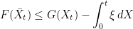
 . It is relatively straightforward to show that (
 will be of the form
  for an increasing right-continuous function
  , so
, so 
 , so can be used as the definition of
  . In the case where X is a semimartingale, integration by parts ensures that this agrees with the stochastic integral
  . Since we now have an interpretation of (
 ,
,
 .
. then,
then,
 .
.
 .
.
 is a measure of the time spent at x. For a continuous time stochastic process, we could try and simply compute the Lebesgue measure of the time at the level,
 and stick there for some time, this makes some sense. However, if X is a standard
  at each positive time, so that that
  defined by (
 as in (
![{{\mathbb E}[\delta(X_s-x)]}](https://s0.wp.com/latex.php?latex=%7B%7B%5Cmathbb+E%7D%5B%5Cdelta%28X_s-x%29%5D%7D&bg=ffffff&fg=000000&s=0&c=20201002) can be interpreted as the probability density of
can be interpreted as the probability density of  evaluated at
 ![\displaystyle L^x_t=\int_0^t\delta(X_s-x)d[X]_s](https://s0.wp.com/latex.php?latex=%5Cdisplaystyle++L%5Ex_t%3D%5Cint_0%5Et%5Cdelta%28X_s-x%29d%5BX%5D_s+&bg=ffffff&fg=000000&s=0&c=20201002)

 of a
of a ![{\int f^{\prime\prime}(X)d[X]}](https://s0.wp.com/latex.php?latex=%7B%5Cint+f%5E%7B%5Cprime%5Cprime%7D%28X%29d%5BX%5D%7D&bg=ffffff&fg=000000&s=0&c=20201002) and, hence, requires
and, hence, requires  can be understood in terms of distributions, and delta functions can appear, which brings local times into the picture. In the opposite direction, which I take in this post, we can try to generalise Ito’s formula and invert this to give a meaning to (
 . For this to make sense, we must assume that
  is almost surely finite at all times, and I will suppose that
  is the filtration generated by W.
 is not almost surely zero). In this case X has exactly the same distribution as W, so cannot be distinguished from the driftless case with
  by looking at the distribution of X alone.
 and
and  . This allows us to back out the drift
  to be the filtration generated by a standard Brownian motion W in
  , and we define
  , can we find an
  such that the filtration generated by
  is smaller than
  , and work with respect to a
  . Then,
  is used to represent the collection of events observable up to and including time n. Stochastic processes will all be real-valued and defined up to almost-sure equivalence. That is, processes X and Y are considered to be the same if
  almost surely for each
  . The projections of a process X are defined as follows.
 , exists if and only if
 ![{{\mathbb E}[\lvert X_n\rvert\,\vert\mathcal{F}_n]}](https://s0.wp.com/latex.php?latex=%7B%7B%5Cmathbb+E%7D%5B%5Clvert+X_n%5Crvert%5C%2C%5Cvert%5Cmathcal%7BF%7D_n%5D%7D&bg=ffffff&fg=000000&s=0&c=20201002) is almost surely finite for each n, in which case
is almost surely finite for each n, in which case![\displaystyle {}^{\rm o}\!X_n={\mathbb E}[X_n\,\vert\mathcal{F}_n].](https://s0.wp.com/latex.php?latex=%5Cdisplaystyle++%7B%7D%5E%7B%5Crm+o%7D%5C%21X_n%3D%7B%5Cmathbb+E%7D%5BX_n%5C%2C%5Cvert%5Cmathcal%7BF%7D_n%5D.+&bg=ffffff&fg=000000&s=0&c=20201002)
 , exists if and only if
 ![{{\mathbb E}[\lvert X_n\rvert\,\vert\mathcal{F}_{n-1}]}](https://s0.wp.com/latex.php?latex=%7B%7B%5Cmathbb+E%7D%5B%5Clvert+X_n%5Crvert%5C%2C%5Cvert%5Cmathcal%7BF%7D_%7Bn-1%7D%5D%7D&bg=ffffff&fg=000000&s=0&c=20201002) is almost surely finite for each n, in which case
is almost surely finite for each n, in which case![\displaystyle {}^{\rm p}\!X_n={\mathbb E}[X_n\,\vert\mathcal{F}_{n-1}].](https://s0.wp.com/latex.php?latex=%5Cdisplaystyle++%7B%7D%5E%7B%5Crm+p%7D%5C%21X_n%3D%7B%5Cmathbb+E%7D%5BX_n%5C%2C%5Cvert%5Cmathcal%7BF%7D_%7Bn-1%7D%5D.+&bg=ffffff&fg=000000&s=0&c=20201002)
 , and only consider real-valued processes. Any two processes are considered to be the same if they are equal
 ![{{\mathbb E}[1_{\{\tau < \infty\}}\lvert X_\tau\rvert\;\vert\mathcal{F}_\tau]}](https://s0.wp.com/latex.php?latex=%7B%7B%5Cmathbb+E%7D%5B1_%7B%5C%7B%5Ctau+%3C+%5Cinfty%5C%7D%7D%5Clvert+X_%5Ctau%5Crvert%5C%3B%5Cvert%5Cmathcal%7BF%7D_%5Ctau%5D%7D&bg=ffffff&fg=000000&s=0&c=20201002) is almost surely finite for each
is almost surely finite for each ![\displaystyle 1_{\{\tau < \infty\}}{}^{\rm o}\!X_\tau={\mathbb E}[1_{\{\tau < \infty\}}X_\tau\,\vert\mathcal{F}_\tau]](https://s0.wp.com/latex.php?latex=%5Cdisplaystyle++1_%7B%5C%7B%5Ctau+%3C+%5Cinfty%5C%7D%7D%7B%7D%5E%7B%5Crm+o%7D%5C%21X_%5Ctau%3D%7B%5Cmathbb+E%7D%5B1_%7B%5C%7B%5Ctau+%3C+%5Cinfty%5C%7D%7DX_%5Ctau%5C%2C%5Cvert%5Cmathcal%7BF%7D_%5Ctau%5D+&bg=ffffff&fg=000000&s=0&c=20201002)
![{{\mathbb E}[1_{\{\tau < \infty\}}\lvert X_\tau\rvert\;\vert\mathcal{F}_{\tau-}]}](https://s0.wp.com/latex.php?latex=%7B%7B%5Cmathbb+E%7D%5B1_%7B%5C%7B%5Ctau+%3C+%5Cinfty%5C%7D%7D%5Clvert+X_%5Ctau%5Crvert%5C%3B%5Cvert%5Cmathcal%7BF%7D_%7B%5Ctau-%7D%5D%7D&bg=ffffff&fg=000000&s=0&c=20201002) is almost surely finite for each
is almost surely finite for each ![\displaystyle 1_{\{\tau < \infty\}}{}^{\rm p}\!X_\tau={\mathbb E}[1_{\{\tau < \infty\}}X_\tau\,\vert\mathcal{F}_{\tau-}]](https://s0.wp.com/latex.php?latex=%5Cdisplaystyle++1_%7B%5C%7B%5Ctau+%3C+%5Cinfty%5C%7D%7D%7B%7D%5E%7B%5Crm+p%7D%5C%21X_%5Ctau%3D%7B%5Cmathbb+E%7D%5B1_%7B%5C%7B%5Ctau+%3C+%5Cinfty%5C%7D%7DX_%5Ctau%5C%2C%5Cvert%5Cmathcal%7BF%7D_%7B%5Ctau-%7D%5D+&bg=ffffff&fg=000000&s=0&c=20201002)
 decreasing to a limit
  ,
,  almost-surely tends to
  , it does not follow that X is right-continuous. As a counterexample, if
  is any continuously distributed random time, then the process
  is not right-continuous. However, so long as the distribution of
  . Two processes are considered to be the same if they are equal
  in probability, for each uniformly bounded sequence
  converges in probability, for each uniformly bounded decreasing sequence
  . In light of such examples, it is even more remarkable that right-continuity and the existence of left and right limits can be determined by just looking at convergence in probability along monotonic sequences of stopping times. Theorem