Pathwise Burkholder-Davis-Gundy Inequalities

As covered earlier in my notes, the Burkholder-David-Gundy inequality relates the moments of the maximum of a local martingale M with its quadratic variation,

$\displaystyle c_p^{-1}{\mathbb E}[[M]^{p/2}_\tau]\le{\mathbb E}[\bar M_\tau^p]\le C_p{\mathbb E}[[M]^{p/2}_\tau].$

(1)

Here, ${\bar M_t\equiv\sup_{s\le t}\lvert M_s\rvert}$ is the running maximum, ${[M]}$ is the quadratic variation, ${\tau}$ is a stopping time, and the exponent ${p}$ is a real number greater than or equal to 1. Then, ${c_p}$ and ${C_p}$ are positive constants depending on p, but independent of the choice of local martingale and stopping time. Furthermore, for continuous local martingales, which are the focus of this post, the inequality holds for all ${p > 0}$ .

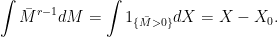
Since the quadratic variation used in my notes, by definition, starts at zero, the BDG inequality also required the local martingale to start at zero. This is not an important restriction, but it can be removed by requiring the quadratic variation to start at ${[M]_0=M_0^2}$ . Henceforth, I will assume that this is the case, which means that if we are working with the definition in my notes then we should add ${M_0^2}$ everywhere to the quadratic variation ${[M]}$ .

In keeping with the theme of the previous post on Doob’s inequalities, such martingale inequalities should have pathwise versions of the form

$\displaystyle c_p^{-1}[M]^{p/2}+\int\alpha dM\le\bar M^p\le C_p[M]^{p/2}+\int\beta dM$

(2)

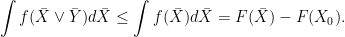
for predictable processes ${\alpha,\beta}$ . Inequalities in this form are considerably stronger than (1), since they apply on all sample paths, not just on average. Also, we do not require M to be a local martingale — it is sufficient to be a (continuous) semimartingale. However, in the case where M is a local martingale, the pathwise version (2) does imply the BDG inequality (1), using the fact that stochastic integration preserves the local martingale property.

Lemma 1 Let X and Y be nonnegative increasing measurable processes satisfying ${X\le Y-N}$ for a local (sub)martingale N starting from zero. Then, ${{\mathbb E}[X_\tau]\le{\mathbb E}[Y_\tau]}$ for all stopping times ${\tau}$ .

Proof: Let ${\tau_n}$ be an increasing sequence of bounded stopping times increasing to infinity such that the stopped processes ${N^{\tau_n}}$ are submartingales. Then,

$\displaystyle {\mathbb E}[1_{\{\tau_n\ge\tau\}}X_\tau]\le{\mathbb E}[X_{\tau_n\wedge\tau}]={\mathbb E}[Y_{\tau_n\wedge\tau}]-{\mathbb E}[N_{\tau_n\wedge\tau}]\le{\mathbb E}[Y_{\tau_n\wedge\tau}]\le{\mathbb E}[Y_\tau].$

Letting n increase to infinity and using monotone convergence on the left hand side gives the result. ⬜

Moving on to the main statements of this post, I will mention that there are actually many different pathwise versions of the BDG inequalities. I opt for the especially simple statements given in Theorem 2 below. See the papers Pathwise Versions of the Burkholder-Davis Gundy Inequality by Bieglböck and Siorpaes, and Applications of Pathwise Burkholder-Davis-Gundy inequalities by Soirpaes, for slightly different approaches, although these papers do also effectively contain proofs of (3,4) for the special case of ${r=1/2}$ . As usual, I am using ${x\vee y}$ to represent the maximum of two numbers.

Theorem 2 Let X and Y be nonnegative continuous processes with ${X_0=Y_0}$ . For any ${0 < r\le1}$ we have,

$\displaystyle (1-r)\bar X^r\le (3-2r)\bar Y^r+r\int(\bar X\vee\bar Y)^{r-1}d(X-Y)$ (3)

and, if X is increasing, this can be improved to,

$\displaystyle \bar X^r\le (2-r)\bar Y^r+r\int(\bar X\vee\bar Y)^{r-1}d(X-Y).$ (4)

If ${r\ge1}$ and X is increasing then,

$\displaystyle \bar X^r\le r^{r\vee 2}\,\bar Y^r+r^2\int(\bar X\vee\bar Y)^{r-1}d(X-Y).$ (5)

Proofs of these inequalities are given below but, for now, some technical points are in order. To interpret the integrals on the right hand side of (3,4,5) using stochastic integration, we should require that X and Y are semimartingales, and that ${(\bar X\vee\bar Y)^{r-1}}$ is ${(X-Y)}$ integrable. When ${r < 1}$ this is not immediate, since the integrand need not be locally bounded. Alternatively, integration by parts can be used to express the integral as

$\displaystyle \int VdZ=VZ-V_0Z_0-\int ZdV,$

(6)

with ${Z=X-Y}$ and ${V=(\bar X\vee\bar Y)^{r-1}}$ . As ${\lvert Z\rvert\le \bar X\vee\bar Y}$ , it can be seen that Z is V-integrable in the pathwise Lebesgue–Stieltjes sense. So, (6) can be used as the definition of the integral, in which case (3,4,5) are valid inequalities for all nonnegative continuous processes with a common initial value. For this reason, it was not required for X and Y to be semimartingales in the statement of theorem 2. In the situation we are interested in, ${(X-Y)}$ will be a continuous local martingale, in which case I show below ${(\bar X\vee\bar Y)^{r-1}}$ is ${(X-Y)}$ -integrable so that the integrals on the right hand side of (3,4,5) are local martingales. If preferred, it can simply be assumed that X and Y start at a strictly positive value, by adding a constant ${\epsilon > 0}$ if necessary, so that the integrands are bounded.

Now consider a continuous semimartingale M starting from zero and ${0 < p <\infty}$ . We can substitute ${X=[M]}$ , ${Y=M^2}$ and ${r=p/2}$ into inequalities (4,5) to obtain,

$\displaystyle [M]^{p/2}\le c_p\bar M^p+a_p\int(\bar M\vee[M]^{1/2})^{p-2}d([M]-M^2).$

(7)

for positive constants ${c_p,a_p}$ . As ${M^2-[M]}$ is a local martingale, lemma 1 implies the left hand side of the BDG inequality (1). Similarly, we can substitute ${X=M^2}$ , ${Y=[M]}$ and ${r=p/2}$ into (3) to get,

$\displaystyle \bar M^p\le C_p[M]^{p/2}+b_p\int(\bar M\vee[M]^{1/2})^{p-2}d(M^2-[M])$

(8)

for positive constants ${C_p,b_p}$ . Lemma 1 then implies the right hand side of the BDG inequality. However, as (3) only applies for ${r < 1}$ , this argument holds for ${p < 2}$ . Unfortunately, when X is not increasing, the results of theorem 2 do not extend to ${r\ge1}$ . In that case, we can make use of the following alternative pathwise inequality which, incidentally, does not require continuity of the process.

Theorem 3 Let X be a semimartingale starting from zero. Then, for any ${p\ge2}$ ,

$\displaystyle \bar X^p\le C_p[X]^{p/2}+\frac12p^2q\int\left(\lvert qX_-\rvert^{p-1}-\bar X_-^{p-1}\right){\rm sgn}(X_-)dX$ (9)

with ${p^{-1}+q^{-1}=1}$ and ${C_p=\left(\tfrac12p(p-1)q^p\right)^{p/2}}$ .

The proof of this, given further below, is a relatively straightforward application of Ito’s lemma and the pathwise Doob inequality. For the non-pathwise approach see, for example, Protter, Chapter IV, theorem 73. We note that applying lemma 1 to the pathwise inequalities (7,8,9) proves the BDG inequality for all values of the exponent.

Corollary 4 For each ${p > 0}$ there exists positive constants ${c_p,C_p}$ satisfying

$\displaystyle c^{-1}_p{\mathbb E}[[M]^{p/2}_\tau]\le{\mathbb E}[\bar M^p_\tau]\le C_p{\mathbb E}[[M]^{p/2}_\tau]$

for all continuous local martingales M and stopping times ${\tau}$ .

The exposition above is not intended to derive the best constants in the BDG inequality. Instead, the aim is to give very simple pathwise versions. However, it is still interesting to note the constants obtained. Starting with the left hand side,

$\displaystyle c_p=\begin{cases} 2-p/2,&{\rm for\ }p\le2,\\ p^2/4,&{\rm for\ }2\le p\le4,\\ (p/2)^{p/2},&{\rm for\ }p\ge4. \end{cases}$

In particular, for the important case of ${p=1}$ we obtain ${c_1=3/2}$ . The optimal constant was derived by Schachermayer and Stebegg to be ${c_1\approx1.27267\ldots}$ , although no simple expression was given for this value. For the right hand BDG inequality, the argument above gives,

$\displaystyle C_p=\begin{cases} (3-p)/(1-p/2),&{\rm for\ }p < 2,\\ (\tfrac12p(p-1)q^p)^{p/2},&{\rm for\ }p\ge 2. \end{cases}$

As p goes to infinity, we have ${C^{1/p}_p=O(p)}$ . This is an optimal growth rate for general cadlag local martingales, although it is possible to improve this to ${O(\sqrt p)}$ for continuous local martingales. These values of ${C_p}$ diverge to infinity as ${p}$ tends to 2 from below, which is a bit unsatisfactory, as we would expect the optimal value of ${C_p}$ to tend to ${C_2=4}$ . This behaviour is a consequence of using inequality (3) for ${p < 2}$ , and switching to a different approach (9) for ${p\ge2}$ . Sharper pathwise inequalities can be obtained, at the expense of having more complicated expressions. For example, for nonnegative continuous processes X and Y with ${X_0=Y_0}$ , combining the approach above with the methods used in the post on pathwise Doob inequalities gives the following alternative to (8) over ${1 \le p \le2}$ ,

$\displaystyle \begin{aligned} \bar X^p\le 2p(3-p)\bar Y^p &+p^2\int(\bar X\vee\bar Y)^{p-2}d(X^2-Y^2)\\ &-2p(p-1)\int\bar X^{p-1}dX. \end{aligned}$

(10)

See lemma 8 below. Substituting ${X=\lvert M\rvert}$ and ${Y=[M]^{1/2}}$ in this gives a pathwise BDG inequality with constant

$\displaystyle C_p=2p(3-p)$

over ${1 \le p\le 2}$ , which is continuous with ${C_2=4}$ .

Proofs of Inequalities

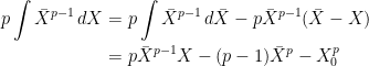
I start by giving the proof of theorem 3 which, as mentioned, is an application of Ito’s formula and the pathwise Doob inequality.

Proof of theorem 3: For brevity, I will set ${\sigma={\rm sgn}(X_-)}$ . We apply Ito’s formula,

$\displaystyle \begin{aligned} \lvert X\rvert^p = & p\int \lvert X\rvert^{p-1}_-\sigma dX+\frac12p(p-1)\int\lvert X\rvert^{p-2}d[X]^{(c)}\\ &\ +\sum\left(\Delta\lvert X\rvert^p-p\lvert X\rvert^{p-1}_-\sigma\Delta X\right)+\lvert X_0\rvert^p. \end{aligned}$

Next, by Taylor’s theorem,

$\displaystyle \Delta\lvert X\rvert^p=p\lvert X\rvert^{p-1}_-\sigma\Delta X+\frac12p(p-1)\lvert x\rvert^{p-2}(\Delta X)^2$

for some ${x}$ lying between ${X_-}$ and ${X}$ . In particular, ${x}$ is bounded by ${\bar X}$ . So, using the fact that ${d[X]=d[X]^{(c)}+(\Delta X)^2}$ we obtain,

$\displaystyle \begin{aligned} \lvert X\rvert^p &\le p\int \lvert X\rvert^{p-1}_-\sigma dX+\frac12p(p-1)\int\bar X^{p-2}d[X]+\lvert X_0\rvert^p\\ &\le p\int \lvert X\rvert^{p-1}_-\sigma dX+\frac12p(p-1)\bar X^{p-2}[X]. \end{aligned}$

We now make use of the pathwise Doob inequality,

$\displaystyle \bar X^p\le q^p\lvert X\rvert^p-pq\int\bar X^{p-1}_-d\lvert X\rvert.$

However, ${d\lvert X\rvert\ge\sigma dX}$ (see lemma 1 of the post on local times), so we can combine the previous two inequalities,

$\displaystyle \bar X^p\le c\bar X^{p-2}[X]+pq\int\left(\lvert qX\rvert^{p-1}_--\bar X^{p-1}_-\right)\sigma dX$

with ${c=p(p-1)q^p/2}$ . The first term on the right hand side can be split into terms only involving ${\bar X}$ and ${[X]}$ respectively by making use of the AM-GM inequality,

$\displaystyle c\bar X^{p-2}[X]\le\frac{p-2}{p}\bar X^p+\frac{2}{p}c^{p/2}[X]^{p/2}.$

Substituting into the previous inequality and rearranging gives (9). ⬜

We move on to proving the inequalities of theorem 2.

Proof of inequality (5): Setting ${Z=r(\bar X\vee\bar Y)^{r-1}}$ for ${r\ge1}$ , using ${Z\ge r\bar X^{r-1}}$ and integration by parts,

$\displaystyle \begin{aligned} \int Z\,d(\bar X-Y) &\ge r\int \bar X^{r-1}d\bar X-\int Z\,dY\\ &= \bar X^r-ZY+\int Y\,dZ-X_0^r+Z_0Y_0\\ &\ge \bar X^r-Z\bar Y \end{aligned}$

When ${\bar X\ge\bar Y}$ , we can use the AM-GM inequality,

$\displaystyle Z\bar Y=r\bar X^{r-1}\bar Y\le (1-1/r)\bar X^r+r^{r-1}\bar Y^r.$

When ${\bar X\le\bar Y}$ then,

$\displaystyle Z\bar Y=r\bar Y^r\le(1-1/r)\bar X^r+r\,\bar Y^r$

In either case, this gives

$\displaystyle \int Z\,d(\bar X-Y)\ge r^{-1}\bar X^r-r^{(r-1)\vee1}\,\bar Y^r$

as required. ⬜

For inequalities (3,4), we start with the following.

Lemma 5 Let X and Y be nonnegative continuous processes. Then, for any ${0 < r \le 1}$ ,

$\displaystyle 0\le r\int (\bar X\vee\bar Y)^{r-1}d(\bar X-X)\le r\bar X^r+(1-r)\bar Y^r-r\bar X^{r-1}X.$ (11)

Proof: Setting ${F(x)=x^r}$ and ${f(x)=F^\prime(x)=rx^{r-1}}$ , apply integration by parts.

$\displaystyle \int f(\bar X\vee\bar Y)d(\bar X-X)=f(\bar X\vee\bar Y)(\bar X-X)-\int(\bar X-X)df(\bar X\vee\bar Y).$

(12)

As ${f}$ is decreasing and ${\bar X-X}$ is nonnegative, both terms on the right are positive, giving the left hand inequality of (11).

The integral on the right hand side of (12) can be split up as

$\displaystyle \int1_{\{\bar Y >\bar X\}}(\bar X-X)df(\bar Y)+\int1_{\{\bar X\ge\bar Y\}}(\bar X-X)df(\bar X).$

The process ${f(\bar X)}$ only increases when ${\bar X=X}$ so, the second integral above vanishes. For more rigour, see the proof of lemma 5 of the previous post. Hence,

$\displaystyle \begin{aligned} \int(\bar X-X)df(\bar X\vee\bar Y) &=\int1_{\{\bar Y > \bar X\}}(\bar X-X)df(\bar Y)\\ &\ge\int\bar Ydf(\bar Y)\\ &=\bar Yf(\bar Y)-Y_0f(Y_0)-\int f(\bar Y) d\bar Y\\ &\ge\bar Yf(\bar Y)-F(\bar Y) \end{aligned}$

Putting this back into (12) and using ${f(\bar X\vee\bar Y)\le r\bar X^{r-1}}$ gives (11). ⬜

Inequalities (3,4) will be obtained by combining the previous result with the following.

Lemma 6 Let X and Y be nonnegative continuous processes. For any ${0 < r\le 1}$ ,

$\displaystyle \bar X^r-X_0^r\ge r\int(\bar X\vee\bar Y)^{r-1}\,d\bar X\ge\bar X^r-(1-r)\bar Y^r-r\bar Y^{r-1}X_0.$ (13)

Proof: Setting ${F(x)=x^r}$ and ${f(x)=F^\prime(x)=rx^{r-1}}$ then, as ${f}$ is decreasing,

$\displaystyle \int f(\bar X\vee\bar Y)d\bar X \le \int f(\bar X) d\bar X = F(\bar X)-F(X_0).$

Next, fixing time ${t}$ , consider the integral

$\displaystyle I\equiv\int_0^t f(\bar X\vee\bar Y)d\bar X \ge \int_0^t f(\bar X\vee\bar Y_t) d\bar X.$

If ${\bar X_t \ge \bar Y_t}$ then, by continuity, there is a time ${s < t}$ with ${\bar X_s=\bar Y_t}$ , and the integral can be written as,

$\displaystyle \begin{aligned} I &\ge f(\bar Y_t)(\bar X_s-X_0) + F(\bar X_t)-F(\bar X_s)\\ &=f(\bar Y_t)(\bar Y_t-X_0)+F(\bar X_t)-F(\bar Y_t) \end{aligned}$

If ${\bar X_t\le\bar Y_t}$ then,

$\displaystyle \begin{aligned} I &\ge f(\bar Y_t)(\bar X_t-X_0)\\ &\ge f(\bar Y_t)(\bar Y_t-X_0)+F(\bar X_t)-F(\bar Y_t), \end{aligned}$

using concavity of ${F}$ , giving (13). ⬜

Inequality (4) is now a simple application of the previous two lemmas.

Proof of inequality (4): Applying the right hand inequality of (13) and the left hand of (13) with X and Y exchanged,

$\displaystyle \begin{aligned} r\int(\bar X\vee\bar Y)^{r-1}d(\bar X-\bar Y) &\ge \bar X^r-(2-r)\bar Y^r+X_0(r\bar Y^{r-1}-X_0^{r-1})\\ &\ge \bar X^r-(2-r)\bar Y^r. \end{aligned}$

The second inequality here is using ${\bar Y\ge Y_0=X_0}$ . Hence, using the left hand inequality of (11) with X and Y exchanged,

$\displaystyle \begin{aligned} r\int(\bar X\vee\bar Y)^{r-1}d(\bar X-Y) &\ge\bar X^r-(2-r)\bar Y^r+\int(\bar X\vee\bar Y)^{r-1}d(\bar Y-Y)\\ &\ge\bar X^r-(2-r)\bar Y^r \end{aligned}$

as required. ⬜

As X is nonnegative, inequality (14) below implies (3), completing the proof of theorem 2.

Lemma 7 Let X and Y be nonnegative continuous processes with ${X_0=Y_0}$ . Then, for ${0 < r\le1}$ ,

$\displaystyle (1-r)\bar X^r+r\bar X^{r-1}X\le(3-2r)\bar Y^r+r\int(\bar X\vee\bar Y)^{r-1}d(X-Y).$ (14)

Proof: Using ${Z=r(\bar X\vee\bar Y)^{r-1}}$ , substitute in inequalities (4) and (11),

$\displaystyle \begin{aligned} \int Z\,d(X-Y) &=\int Z\,d(\bar X-Y) -\int Z\,d(\bar X-X)\\ &\ge \bar X^r-(2-r)\bar Y^r-r\bar X^r-(1-r)\bar Y^r+r\bar X^{r-1}X. \end{aligned}$

as required. ⬜

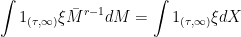
We finally give the proof of inequality (10).

Lemma 8 Let X and Y be nonnegative continuous processes with ${X_0=Y_0}$ . Then, for ${1 \le p \le 2}$ ,

$\displaystyle \begin{aligned} \bar X^p\le 2p(3-p)\bar Y^p &+p^2\int(\bar X\vee\bar Y)^{p-2}d(X^2-Y^2)\\ &-2p(p-1)\int\bar X^{p-1}dX. \end{aligned}$

Proof: Substitute ${X^2,Y^2,p/2}$ for ${X,Y,r}$ in (14),

$\displaystyle (1-p/2)\bar X^p+\frac p2\bar X^{p-2}X^2\le(3-p)\bar Y^p+\frac p2\int(\bar X\vee\bar Y)^{p-2}d(X^2-Y^2).$

(15)

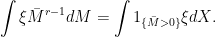
Apply lemma 5 from the post on pathwise Doob inequalities, with ${h(x)=px^{p-1}}$ ,

$\displaystyle \begin{aligned} p\int \bar X^{p-1}\,dX &=p\int \bar X^{p-1}\,d\bar X-p\bar X^{p-1}(\bar X-X)\\ &=p\bar X^{p-1}X-(p-1)\bar X^p-X_0^p \end{aligned}$

Noting that ${X_0}$ is nonnegative, we can multiply through by ${2(p-1)}$ and combine with the AM-GM inequality,

$\displaystyle \begin{aligned} 2p(p-1)\int\bar X^{p-1}dX &\le 2(p-1)\bar X^{p/2}(p\bar X^{p/2-1}X)-2(p-1)^2\bar X^p\\ &\le(p-1)^2\bar X^p +p^2\bar X^{p-2}X^2-2(p-1)^2\bar X^p\\ &=p^2\bar X^{p-2}X^2 -(p-1)^2\bar X^p. \end{aligned}$

Substituting back into (15), after multiplying through by ${2p}$ , gives the result. ⬜

Integrability

Finally for this post, I show that the integrals on the right hand side of (3,4,5) are well-defined as stochastic integrals, in the case where ${X-Y}$ is a local martingale.

Lemma 9 Let M be a continuous local martingale and ${r > 0}$ . Then, ${\bar M^{r-1}}$ is M-integrable.

Proof: Since the result is immediate for ${r\ge1}$ , we consider ${0 < r < 1}$ . As ${\lvert M\rvert\le\bar M}$ and,

$\displaystyle \int\bar Md\bar M^{r-1}=(r-1)\int\bar M^{r-1}d\bar M=(1-1/r)(\bar M^r-\bar M_0^r),$

we see that M is ${\bar M^{r-1}}$ -integrable in the Lebesgue-Stieltjes sense. So, we can define

$\displaystyle X=\bar M^{r-1}M-\int M d\bar M^{r-1}.$

For any ${K > 0}$ , let ${\tau=\inf\{t\ge0\colon\lvert M_t\rvert\ge K\}}$ . Using integration by parts,

$\displaystyle \begin{aligned} \int1_{(\tau,\infty)} \bar M^{r-1} dM &=1_{[\tau,\infty)}\bar M^{r-1}M-1_{\{\tau=0\}}M_0^r-\int Md(1_{[\tau,\infty)}\bar M^{r-1})\\ &=1_{[\tau,\infty)}(\bar M^{r-1}M-M_\tau\bar M^{r-1}_\tau)-\int1_{[\tau,\infty)}Md\bar M^{r-1}\\ &=X-X^\tau \end{aligned}$

So, ${X-X^\tau}$ is a local martingale. Letting K decrease to zero, then ${X^\tau}$ converges uniformly to the constant process ${X_0}$ , so that X is a local martingale. Let ${\xi \not= 0}$ be a bounded predictable process such that ${\xi\bar M^{r-1}}$ is bounded. Then, integrating the identity above,

$\displaystyle \int1_{(\tau,\infty)}\xi\bar M^{r-1}dM = \int1_{(\tau,\infty)}\xi dX$

We can now let K decrease to zero and use bounded convergence to obtain,

$\displaystyle \int\xi\bar M^{r-1}dM=\int1_{\{\bar M > 0\}}\xi dX.$

Integrating ${\xi^{-1}}$ with respect to both sides shows that ${\bar M^{r-1}}$ is M-integrable with,

$\displaystyle \int\bar M^{r-1}dM = \int1_{\{\bar M > 0\}}dX=X-X_0.$

⬜

Corollary 10 Let X and Y be adapted nonnegative continuous processes such that ${X-Y}$ is a local martingale. Then, for any ${r > 0}$ , ${(\bar X\vee\bar Y)^{r-1}}$ is ${(X-Y)}$ -integrable.

Proof: As the result is immediate for ${r\ge1}$ , consider ${0 < r < 1}$ . Setting ${M=X-Y}$ , then, ${(\bar X\vee\bar Y)^{r-1}\le\bar M^{r-1}}$ , so the result follows from lemma 9. ⬜

	Harry on Filtrations and Adapted P…
	Anonymous on Analytic Sets
	Daniel on Analytic Sets
	Sid on Martingale Convergence
	northwiz on Preservation of the Local Mart…
	George Lowther on Martingale Convergence
	Sid on Martingale Convergence
	George Lowther on The Burkholder-Davis-Gundy Ine…
	George Lowther on Preservation of the Local Mart…
	northwiz on Preservation of the Local Mart…

Pathwise Burkholder-Davis-Gundy Inequalities

Proofs of Inequalities

Integrability

Published by George Lowther

Leave a Reply Cancel reply

Proofs of Inequalities

Integrability

Like this:

Related

Published by George Lowther

Leave a Reply Cancel reply