The Generalized Ito Formula

Recall that Ito’s lemma expresses a twice differentiable function ${f}$ applied to a continuous semimartingale ${X}$ in terms of stochastic integrals, according to the following formula

$\displaystyle f(X) = f(X_0)+\int f^\prime(X)\,dX + \frac{1}{2}\int f^{\prime\prime}(X)\,d[X].$

(1)

In this form, the result only applies to continuous processes but, as I will show in this post, it is possible to generalize to arbitrary noncontinuous semimartingales. The result is also referred to as Ito’s lemma or, to distinguish it from the special case for continuous processes, it is known as the generalized Ito formula or generalized Ito’s lemma.

If equation (1) is to be extended to noncontinuous processes then, there are two immediate points to be considered. The first is that if the process ${X}$ is not continuous then it need not be a predictable process, so ${f^\prime(X),f^{\prime\prime}(X)}$ need not be predictable either. So, the integrands in (1) will not be ${X}$ -integrable. To remedy this, we should instead use the left limits ${X_{t-}}$ in the integrands, which is left-continuous and adapted and therefore is predictable. The second point is that the jumps of the left hand side of (1) are equal to ${\Delta f(X)}$ and, on the right, they are ${f^\prime(X_-)\Delta X+\frac{1}{2}f^{\prime\prime}(X_-)\Delta X^2}$ . There is no reason that these should be equal, and (1) cannot possibly hold in general. To fix this, we can simply add on the correction to the jump terms on the right hand side,

$\displaystyle \setlength\arraycolsep{2pt} \begin{array}{rl} \displaystyle f(X_t) =&\displaystyle f(X_0)+\int_0^t f^\prime(X_-)\,dX + \frac{1}{2}\int_0^t f^{\prime\prime}(X_-)\,d[X]\smallskip\\ &\displaystyle +\sum_{s\le t}\left(\Delta f(X_s)-f^\prime(X_{s-})\Delta X_s-\frac{1}{2}f^{\prime\prime}(X_{s-})\Delta X_s^2\right). \end{array}$

(2)

By using a second order Taylor expansion of ${f}$ , the term inside the summation is almost surely bounded by a multiple of ${\Delta X^2}$ . As it was previously shown that the jumps of a semimartingale satisfy ${\sum_{s\le t}\Delta X^2_s<\infty}$ , the summation above is guaranteed to be absolutely convergent. So, equation (2) makes sense, and the jump sizes on both sides agree. In fact, (2) is true for for all semimartingales, and this is precisely the generalized Ito formula for one dimensional processes.

Before giving the full statement, it helps to introduce a bit of notation to simplify things a bit. Any FV process ${V}$ can be split into two parts. Its purely discontinuous part is the sum of its jumps, ${V^d_t=\sum_{s\le t}\Delta V_s}$ , and its purely continuous part is ${V^c=V-V^d}$ . In particular, I will make use of the purely continuous parts of the quadratic variation and covariations of semimartingales ${X,Y}$

$\displaystyle \setlength\arraycolsep{2pt} \begin{array}{rl} \displaystyle [X]^c_t&\displaystyle\equiv [X]_t-\sum_{s\le t}\Delta X_s^2,\smallskip\\ \displaystyle [X,Y]^c_t&\displaystyle\equiv [X,Y]_t-\sum_{s\le t}\Delta X_s\Delta Y_s. \end{array}$

Note that, by canceling with the quadratic term ${\frac{1}{2}f^{\prime\prime}(X_-)\Delta X^2_s}$ in the summation, the quadratic variation ${[X]}$ in equation (2) can be replaced by its continuous part. This simplifies the equations a bit.

Next, any jointly measurable process ${H_t}$ , which is only ever nonzero on a countable set of times and satisfies ${\sum_{s\le t}\vert H_s\vert<\infty}$ , can be alternatively be considered as a differential. This is done by simply replacing integration with summation. That is,

$\displaystyle dY = H\ \iff\ Y_t = Y_0+\sum_{s\le t}H_s.$

This notation enables equation (2) to be expressed in differential notation. Also, the continuous part of the quadratic covariation ${[X,Y]}$ can be written as ${d[X,Y]^c=d[X,Y]-\Delta X\Delta Y}$ .

A d-dimensional process ${X=(X^1,\ldots,X^d)}$ is said to be a semimartingale if each of its components ${X^i}$ are semimartingales and finally, as in the previous post, I am using the summation convention where indices which occur twice in a single term are summed over. The full statement of the generalized Ito formula using differential notation is then as follows.

Theorem 1 (Generalized Ito Formula) Let ${X=(X^1,\ldots,X^d)}$ be a d-dimensional semimartingale such that ${X_t,X_{t-}}$ take values in an open subset ${U\subseteq{\mathbb R}^d}$ . Then, for any twice continuously differentiable function ${f\colon U\rightarrow{\mathbb R}}$ , ${f(X)}$ is a semimartingale and,

$\displaystyle \setlength\arraycolsep{2pt} \begin{array}{rl} \displaystyle df(X) =&\displaystyle D_if(X_-)\,dX^i + \frac{1}{2}D_{ij}f(X)\,d[X^i,X^j]^c\smallskip\\ &\displaystyle + \left(\Delta f(X) - D_if(X_-)\Delta X^i\right). \end{array}$ (3)

The final two terms on the right hand side of (3) are FV processes. Sometimes, we are only concerned about describing a process up to a finite variation term, in which case the following much simplified version of Ito’s formula can be useful.

Corollary 2 Let ${X=(X^1,\ldots,X^d)}$ be a d-dimensional semimartingale and ${f\colon{\mathbb R}^d\rightarrow{\mathbb R}}$ be twice continuously differentiable. Then,

$\displaystyle f(X)=\int D_if(X_-)\,dX^i + V$

for some FV process ${V}$ .

For example, FV processes only contribute pure jump terms to quadratic covariations and therefore do not contribute at all to the continuous part. So, Corollary 2 has the following consequence.

Corollary 3 Let ${X=(X^1,\ldots,X^d)}$ be a d-dimensional semimartingale and ${f\colon{\mathbb R}^d\rightarrow{\mathbb R}}$ be twice continuously differentiable. Then,

$\displaystyle \left[f(X),Y\right]^c=\int D_if(X)\,d[X^i,Y]^c.$

for any semimartingale ${Y}$ .

Example: The Doléans exponential

As previously mentioned, the Doléans exponential of a semimartingale ${X}$ is the solution to the integral equation

$\displaystyle U=1+\int U_-\,dX,$

and is denoted by ${\mathcal{E}(X)}$ . This can be solved with the help of the generalized Ito formula. The continuous part of the quadratic variation satisfies ${d[U]^c=U_-\,d[X]^c}$ and the jumps are ${\Delta U=U_-\Delta X}$ . Assuming that ${U}$ remains positive, the generalized Ito formula gives,

$\displaystyle \setlength\arraycolsep{2pt} \begin{array}{rl} \displaystyle d\log(U) &\displaystyle= U_-^{-1}\,dU-\frac{1}{2}U_-^{-2}\,d[U]^c+(\Delta \log(U)-U_{-}^{-1}\Delta U)\smallskip\\ &\displaystyle=dX-\frac{1}{2}\,d[X]^c+(\log(1+\Delta X)-\Delta X). \end{array}$

(4)

Here, I have applied the identity

$\displaystyle \Delta\log(U)=\log(1+U_-^{-1}\Delta U)=\log(1+\Delta X).$

Integrating (4) gives,

$\displaystyle \log(U_t) =X_t-X_0-\frac{1}{2}[X]^c _t+\sum_{s\le t}(\log(1+\Delta X_s)-\Delta X_s).$

Exponentiating gives the following formula for the Doléans exponential of a general semimartingale

$\displaystyle \mathcal{E}(X)_t = \exp\left(X_t-X_0-\frac{1}{2}[X]^c_t\right)\prod_{s\le t}e^{-\Delta X_s}(1+\Delta X_s).$

(5)

This gives the general form for the Doléans exponential, but, a brief comment on the derivation above is in order. In order to apply the logarithm, it was assumed that the process remains positive. However, from (5) it can be seen that it goes negative or zero if there is a jump ${\Delta X\le -1}$ . This problem is not difficult to fix by splitting the process ${X}$ into two terms, one with the jumps less than -1 removed and the other only containing such jumps. Then, the argument above holds when applied to the first term, and it is easily verified that equation (5) remains true after adding in the second, piecewise constant, term.

Proof of Ito’s Formula

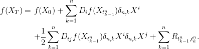
Writing out equation (3) in integral form, and substituting in the quadratic covariation rather than just its continuous part gives the following,

$\displaystyle \setlength\arraycolsep{2pt} \begin{array}{rl} \displaystyle f(X_T) =&\displaystyle f(X_0)+\int_0^TD_if(X_-)\,dX^i + \frac{1}{2}\int_0^T D_{ij}f(X_-)\,d[X^i,X^j]\smallskip\\ &\displaystyle + \sum_{t\le T}\left(\Delta f(X_t) - D_if(X_{t-})\Delta X^i_t-\frac{1}{2}D_{ij}f(X_{t-})\Delta X^i_t\Delta X^j_t\right). \end{array}$

(6)

We now prove this formula. As the terms on the right hand side are all FV processes or stochastic integrals, this also shows that ${f(X)}$ is a semimartingale.

For any times ${s\le t}$ , writing ${\delta X\equiv X_t-X_s}$ , a Taylor expansion to second order gives

$\displaystyle f(X_t) = f(X_s) + D_if(X_s)\delta X^i+\frac{1}{2}D_{ij}f(X_s)\delta X^i\delta X^j + R_{s,t}.$

(7)

The set ${\{X_{t-},X_t\colon t\le T\}}$ is almost surely a closed and bounded subset of ${U}$ , for each time ${T}$ . It follows that the remainder term ${R_{s,t}}$ is almost surely of size ${o(\Vert X_t-X_s\Vert^2)}$ uniformly over the interval ${[0,T]}$ . So, ${\Vert X_t-X_s\Vert^{-2}R_{s,t}\rightarrow 0}$ whenever ${\Vert X_t-X_s\Vert\rightarrow 0}$ over ${s,t\in[0,T]}$ .

Now, for a given integer n, partition the interval ${[0,T]}$ into n equal segments. That is, set ${t^n_k=kT/n}$ for ${k=0,1,\ldots,n}$ . Using the notation ${\delta_{n,k}X\equiv X_{t^n_k}-X_{t^n_{k-1}}}$ , sum (7) over the intervals ${(t^n_{k-1},t^n_k)}$ ,

$\displaystyle \setlength\arraycolsep{2pt} \begin{array}{rl} \displaystyle f(X_T) = &\displaystyle f(X_0) + \sum_{k=1}^n D_if(X_{t^n_{k-1}})\delta_{n,k}X^i\smallskip\\ &\displaystyle+ \frac{1}{2}\sum_{k=1}^nD_{ij}f(X_{t^n_{k-1}})\delta_{n,k}X^i\delta_{n,k}X^j + \sum_{k=1}^n R_{t^n_{k-1},t^n_k}. \end{array}$

(8)

The aim is to show that this converges to equation (6) in the limit as n goes to infinity. The first two summations have already been dealt with in the previous post, where it was shown that the following limits hold in probability as ${n\rightarrow\infty}$ .

$\displaystyle \begin{array}{rl} &\displaystyle\sum_{k=1}^n D_if(X_{t^n_{k-1}})\delta_{n,k}X^i\rightarrow \int_0^T D_if(X_-)\,dX^i,\smallskip\\ &\displaystyle\sum_{k=1}^nD_{ij}f(X_{t^n_{k-1}})\delta_{n,k}X^i\delta_{n,k}X^j\rightarrow\int_0^TD_{ij}f(X_-)\,d[X^i,X^j]. \end{array}$

So, the first three terms on the right hand side of equation (8) do indeed converge to the first three terms on the right hand side of (6). It only remains to show that the remainder term ${\sum_kR_{t^n_{k-1},t^n_k}}$ converges to the summation in (6). Note that the remainders ${R_{s,t}}$ satisfy

$\displaystyle \setlength\arraycolsep{2pt} \begin{array}{rl} \displaystyle R_{s,t} &\displaystyle= f(X_t)-f(X_s)-D_{i}f(X_s)\delta X^i -\frac{1}{2}D_{ij}f(X_s)\delta X^i\delta X^j\smallskip\\ &\displaystyle\rightarrow\Delta f(X_u)-D_if(X_{u-})\Delta X^i_u - \frac{1}{2}D_{ij}f(X_{u-})\Delta X^i_u\Delta X^j_u \end{array}$

as ${s,t\rightarrow u}$ with ${s<u\le t}$ . The result is then given by the following.

Lemma 4 Let ${X}$ be a d-dimensional semimartingale and ${R_{s,t}}$ be of size ${o(\Vert X_t-X_s\Vert^2)}$ uniformly over the interval ${[0,T]}$ . Suppose, furthermore, that there is a process ${r_u}$ satisfying

$\displaystyle R_{s,t}\rightarrow r_u$ (9)

as ${s,t\rightarrow u}$ over ${s<u\le t}$ for all times ${u}$ .

Then ${\sum_{t\le T}\vert r_t\vert}$ is almost surely finite and,

$\displaystyle \sum_{k=1}^n R_{t^n_{k-1},t^n_k}\rightarrow\sum_{t\le T}r_t$ (10)

in probability as ${n\rightarrow\infty}$ .

Proof: The condition that ${R_{s,t}}$ is of size ${o(\Vert X_t-X_s\Vert^2)}$ means that, for ${\epsilon>0}$ , the random variables

$\displaystyle U(\epsilon)\equiv\sup\left\{\Vert X_t-X_s\Vert^{-2}R_{s,t}\colon s,t\in[0,T],\ 0<\Vert X_t-X_s\Vert\le \epsilon\right\}$

tend to zero in the limit ${\epsilon\rightarrow 0}$ . In particular, ${\vert R_{s,t}\vert \le V \Vert X_t-X_s\Vert^2}$ for some random variable V and, by taking limits, ${\vert r_u\vert\le V\Vert\Delta X_u\Vert^2}$ giving,

$\displaystyle \sum_{t\le T}\vert r_t\vert \le V\sum_{t\le T}\Vert\Delta X_t\Vert^2\le V [X^i,X^i]_T<\infty.$

I now split the proof up into two cases. First, where ${R_{s,t}}$ is zero for small values of ${X_t-X_s}$ , and then when it is zero for large values of ${X_t-X_s}$ .

So, suppose that ${R_{s,t}=0}$ whenever ${\Vert X_t-X_s\Vert < \epsilon}$ , for some positive ${\epsilon}$ . Then, limit (10) holds almost surely. In fact, for large enough n, the terms ${R_{t^n_{k-1},t^n_k}}$ will all be zero except for those intervals ${(t^n_{k-1},t^n_k]}$ in which ${X}$ has a jump of magnitude at least ${\epsilon}$ . So it reduces to a finite sum, and the limit follows from applying (9) to each term.

Now, suppose that ${R_{s,t}=0}$ whenever ${\Vert X_t-X_s\Vert \ge \epsilon}$ . Then,

$\displaystyle \left\vert\sum_{k=1}^nR_{t^n_{k-1},t^n_k}\right\vert\le U(\epsilon)\sum_{k=1}^n\Vert\delta_{n,k}X\Vert^2 \rightarrow U(\epsilon)[X^i,X^i]_T$

(11)

in probability as ${n\rightarrow \infty}$ .

We can now piece these cases together. For any ${\epsilon>0}$ , choose a continuous function ${\theta\colon{\mathbb R}_+\rightarrow[0,1]}$ such that ${\theta(x)}$ is equal to 1 for ${x\ge\epsilon}$ and equal to zero for ${x<\epsilon/2}$ .

Applying limit (10) to the terms ${\theta(\Vert X_t-X_s\Vert)R_{s,t}}$ and (11) to ${(1-\theta(\Vert X_t-X_s\Vert))R_{s,t}}$ gives the following,

$\displaystyle \setlength\arraycolsep{2pt} \begin{array}{rcl} \displaystyle\left\vert \sum_{k=1}^n R_{t^n_{k-1},t^n_k}-\sum_{t\le T}r_t\right\vert &\displaystyle\le &\displaystyle\left\vert \sum_{k=1}^n \theta(\Vert \delta_{n,k}X\Vert)R_{t^n_{k-1},t^n_k}-\sum_{t\le T}\theta(\Vert\Delta X_t\Vert)r_t\right\vert\smallskip\\ &&\displaystyle+ U(\epsilon)\sum_{k=1}^n\Vert\delta_{n,k}X\Vert^2+\sum_{t\le T}1_{\{\Vert\Delta X_t\Vert<\epsilon\}}\vert r_t\vert\smallskip\\ &\displaystyle\rightarrow &\displaystyle U(\epsilon)[X^i,X^i]_T + \sum_{t\le T}1_{\{\Vert \Delta X_t\Vert<\epsilon\}}\vert r_t\vert. \end{array}$

in probability as ${n\rightarrow \infty}$ . By choosing ${\epsilon}$ small, the right hand side can be made as small as we like, showing that

$\displaystyle \left\vert \sum_{k=1}^n R_{t^n_{k-1},t^n_k}-\sum_{t\le T}r_t\right\vert\rightarrow 0$

in probability as ${n\rightarrow\infty}$ . ⬜

10 thoughts on “The Generalized Ito Formula”

Dominic says:

25 December 12 at 7:01 AM

Hi, I think there’s a minus sign missing from the integrand in theorem 1.

Is there any reason to not just give the formula as $df(X) = D_if(X_-)dX^{i,c} + D_{ij}f(X_-)d[X^i,X^j]^c + \sum_{s\le t}\Delta f(X_s)$ ?

1. Dominic says:
  
  25 December 12 at 7:09 AM
  
  Oh right, the summation term needn’t converge, so we need the compensation terms from the first integral at least. I see.
  
Tom Mike says:

8 July 17 at 8:03 PM

Hello,

When the function f is one dimensional, it is easy to understand what is \Delta f (X_s) = f (X_s + jump ) – f( X_s). But what is the signification of \Delta f (X_s) when f is a two dimensional function for example?

Is it \Delta f (X_s, Y_s) = f(X_s + jump of X_s, Y_s + jump of Y_s) – f ( X_s, Y_s) ?
or \Delta f (X_s, Y_s) = f(X_s + jump of X_s, jump of Y_s) – f ( X_s, Y_s) + (X_s, jump of Y_s) – f ( X_s, Y_s + jump of Y_s).

Thank you !

Anonymous says:

28 March 18 at 9:07 PM

Hi,

Thanks for this great answer. We wanted to cite this generalized Ito’s lemma in our paper and were wondering what is a good reference to cite.

Anonymous says:

15 January 21 at 12:38 PM

Dear George,

How do we know that the function $\sum_{t \leq T}r_t$ in Lemma 4 is measurable ?

1. George Lowther says:
  
  18 January 21 at 2:51 PM
  
  Use the fact that $r_t$ is only ever zero at times at which X jumps. So, there is a sequence of random times (actually, stopping times) Tn which includes all the times when r is nonzero. Hence, the sum can be written as $\sum_{n=1}^\infty 1_{\{T_n\le T\}}r_{T_n}$ , which is a countable sum of measurable terms, so is measurable.
  
  Alternatively, the result itself implies that this is a limit (in probability or almost sure, either works) of measurable random variables, so is measurable.
  
Anonymous says:

17 January 21 at 11:31 AM

Dear George,

Since $U(\epsilon) \sum_{k = 1}^{n} \Vert\delta_{n,k}X\Vert^2 \le U(\epsilon) [X^i,X^i]$ can’t we put in the conclusion of lemma 4 the stronger statement that $\sum_{k = 1}^nR_{t^n_{k - 1},t^n_k} \rightarrow \sum_{t \leq T}r_t$ almost sure instead of probability ?

1. George Lowther says:
  
  18 January 21 at 2:54 PM
  
  Actually, I think you can. Convergence in probability is sufficient for our purposes, but the stronger statement should also hold.
  
leejulian6702 says:

27 January 22 at 1:45 PM

I can’t understand why the final terms in (3) or (6) FV processes. Could you explain this to me?

1. George Lowther says:
  
  20 February 22 at 4:09 PM
  
  The final terms are a sum over discrete jump terms. These are absolutely convergent (they must be for the sum to make sense), so give FV processes.
  As f is twice differentiable, these terms are all of order $(\Delta X)^2$ , which has a finite sum for any semimartingale X.

	George Lowther on Filtrations and Adapted P…
	faceet on Filtrations and Adapted P…
	George Lowther on Filtrations and Adapted P…
	facet on Filtrations and Adapted P…
	Zoltan on Class (D) Processes
	Zoltan on Class (D) Processes
	ARS on Stopping Times and the Debut…
	George Lowther on Upcrossings, Downcrossings, an…
	George Lowther on Stopping Times and the Debut…
	ARS on Stopping Times and the Debut…

The Generalized Ito Formula

Example: The Doléans exponential

Proof of Ito’s Formula

Published by George Lowther

10 thoughts on “The Generalized Ito Formula”

Leave a Reply Cancel reply

Example: The Doléans exponential

Proof of Ito’s Formula

Like this:

Related

Published by George Lowther

10 thoughts on “The Generalized Ito Formula”

Leave a Reply Cancel reply