Bessel Processes

A random variable ${N=(N^1,\ldots,N^n)}$ has the standard n-dimensional normal distribution if its components ${N^i}$ are independent normal with zero mean and unit variance. A well known fact of such distributions is that they are invariant under rotations, which has the following consequence. The distribution of ${Z\equiv\Vert N+\boldsymbol{\mu}\Vert^2}$ is invariant under rotations of ${\boldsymbol{\mu}\in{\mathbb R}^n}$ and, hence, is fully determined by the values of ${n\in{\mathbb N}}$ and ${\mu=\Vert\boldsymbol{\mu}\Vert^2\in{\mathbb R}_+}$ . This is known as the noncentral chi-square distribution with n degrees of freedom and noncentrality parameter ${\mu}$ , and denoted by ${\chi^2_n(\mu)}$ . The moment generating function can be computed,

$\displaystyle M_Z(\lambda)\equiv{\mathbb E}\left[e^{\lambda Z}\right]=\left(1-2\lambda\right)^{-\frac{n}{2}}\exp\left(\frac{\lambda\mu}{1-2\lambda}\right),$

(1)

which holds for all ${\lambda\in{\mathbb C}}$ with real part bounded above by 1/2.

A consequence of this is that the norm ${\Vert B_t\Vert}$ of an n-dimensional Brownian motion B is Markov. More precisely, letting ${\mathcal{F}_t=\sigma(B_s\colon s\le t)}$ be its natural filtration, then ${X\equiv\Vert B\Vert^2}$ has the following property. For times ${s<t}$ , conditional on ${\mathcal{F}_s}$ , ${X_t/(t-s)}$ is distributed as ${\chi^2_n(X_s/(t-s))}$ . This is known as the `n-dimensional’ squared Bessel process, and denoted by ${{\rm BES}^2_n}$ .

A Poisson process sample path — Figure 1: Squared Bessel processes of dimensions n=1,2,3

Alternatively, the process X can be described by a stochastic differential equation (SDE). Applying integration by parts,

$\displaystyle dX = 2\sum_iB^i\,dB^i+\sum_id[B^i].$

(2)

As the standard Brownian motions have quadratic variation ${[B^i]_t=t}$ , the final term on the right-hand-side is equal to ${n\,dt}$ . Also, the covarations ${[B^i,B^j]}$ are zero for ${i\not=j}$ from which it can be seen that

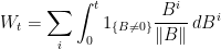
$\displaystyle W_t = \sum_i\int_0^t1_{\{B\not=0\}}\frac{B^i}{\Vert B\Vert}\,dB^i$

is a continuous local martingale with ${[W]_t=t}$ . By Lévy’s characterization, W is a Brownian motion and, substituting this back into (2), the squared Bessel process X solves the SDE

$\displaystyle dX=2\sqrt{X}\,dW+ndt.$

(3)

The standard existence and uniqueness results for stochastic differential equations do not apply here, since ${x\mapsto2\sqrt{x}}$ is not Lipschitz continuous. It is known that (3) does in fact have a unique solution, by the Yamada-Watanabe uniqueness theorem for 1-dimensional SDEs. However, I do not need and will not make use of this fact here. Actually, uniqueness in law follows from the explicit computation of the moment generating function in Theorem 5 below.

Although it is nonsensical to talk of an n-dimensional Brownian motion for non-integer n, Bessel processes can be extended to any real ${n\ge0}$ . This can be done either by specifying its distributions in terms of chi-square distributions or by the SDE (3). In this post I take the first approach, and then show that they are equivalent. Such processes appear in many situations in the theory of stochastic processes, and not just as the norm of Brownian motion. It also provides one of the relatively few interesting examples of stochastic differential equations whose distributions can be explicitly computed.

The ${\chi^2_n(\mu)}$ distribution generalizes to all real ${n\ge0}$ , and can be defined as the unique distribution on ${{\mathbb R}_+}$ with moment generating function given by equation (1). If ${Z_1\sim\chi_m(\mu)}$ and ${Z_2\sim\chi_n(\nu)}$ are independent, then ${Z_1+Z_2}$ has moment generating function ${M_{Z_1}(\lambda)M_{Z_2}(\lambda)}$ and, therefore, has the ${\chi^2_{m+n}(\mu+\nu)}$ distribution. That such distributions do indeed exist can be seen by constructing them. The ${\chi^2_n(0)}$ distribution is a special case of the Gamma distribution and has probability density proportional to ${x^{n/2-1}e^{-x/2}}$ . If ${Z_1,Z_2,\ldots}$ is a sequence of independent random variables with the standard normal distribution and T independently has the Poisson distribution of rate ${\mu/2}$ , then ${\sum_{i=1}^{2T}Z_i^2\sim\chi_0^2(\mu)}$ , which can be seen by computing its moment generating function. Adding an independent ${\chi^2_n(0)}$ random variable Y to this produces the ${\chi^2_n(\mu)}$ variable ${Z\equiv Y+\sum_{i=1}^{2T}Z_i^2}$ .

The definition of squared Bessel processes of any real dimension ${n\ge0}$ is as follows. We work with respect to a filtered probability space ${(\Omega,\mathcal{F},\{\mathcal{F}_t\}_{t\ge0},{\mathbb P})}$ .

Definition 1 A process X is a squared Bessel process of dimension ${n\ge0}$ if it is continuous, adapted and, for any ${s<t}$ , conditional on ${\mathcal{F}_s}$ , ${X_t/(t-s)}$ has the ${\chi^2_n\left(X_s/(t-s)\right)}$ distribution.

Substituting in expression (1) for the moment generating function, this definition is equivalent to X being a continuous adapted process such that, for all times ${s\le t}$ ,

$\displaystyle {\mathbb E}\left[e^{-\lambda X_t}\;\middle\vert\;\mathcal{F}_s\right]=\left(1+2\lambda(t-s)\right)^{-\frac{n}{2}}\exp\left(\frac {-\lambda X_s}{1+2\lambda(t-s)}\right).$

(4)

This holds for all ${\lambda\in{\mathbb C}}$ with nonnegative real part. Also, if the filtration is not specified, then a process X is a Bessel process if it satisfies Definition 1 with respect to its natural filtration ${\mathcal{F}_t=\sigma(X_s\colon s\le t)}$ .

Note that we have not yet shown that Bessel processes for arbitrary non-integer ${n\ge0}$ are well-defined. Definition 1 specifies the properties that such processes must satisfy, but this does not guarantee their existence. It is not difficult to show that (4) determines a Markov transition function, so that the Chapman-Kolmogorov identity is satisfied. In fact, as I show below, it is Feller. See Lemma 9 below, where the existence of continuous modifications is also proven.

For now, let us determine some of the properties of Bessel processes. There are some properties which can be stated directly from the definition. The fact that the sum of independent ${\chi^2_m(\mu)}$ and ${\chi^2_n(\nu)}$ distributed random variables has the ${\chi^2_{m+n}(\mu+\nu)}$ distribution gives the following result for sums of Bessel processes.

Lemma 2 Suppose that X and Y are independent ${{\rm BES}^2_m}$ and ${{\rm BES}^2_n}$ processes respectively. Then, X+Y is a ${{\rm BES}^2_{m+n}}$ process.

Next, Definition 1 only referred to the ratio between the process X and the time increments. So, scaling the time axis and the process values by the same factor leaves the ${{\rm BES}^2_n}$ property unchanged.

Lemma 3 Let X be a ${{\rm BES}^2_n}$ process and ${c>0}$ be constant. Then, ${c^{-1}X_{ct}}$ is also a ${{\rm BES}^2_n}$ process.

Standard Brownian motion X satisfies a time reversal symmetry whereby ${tX_{\frac1t}}$ is also a standard Brownian motion, as can be determined by computing covariances. It follows that if X is a ${{\rm BES}^2_n(0)}$ process for integer n, then so is ${t^2X_{\frac1t}}$ , as we can see by expressing it as the sum of squares of independent Brownian motions. This time reversal symmetry extends to Bessel processes of non-integer dimension, as we would expect.

Lemma 4 If X is a ${{\rm BES}^2_n(0)}$ process then so is ${Y_t=t^2X_{\frac1t}}$ .

Proof: As Y is a deterministic time change and scaling of the Markov process X, it is also Markov. Hence, we just need to show that X and Y have the same pairwise distributions. For times ${0 < s < t}$ , we compute the joint moment generating function of ${(X_s,X_t)}$ by applying (4) twice,

$\displaystyle \begin{aligned} {\mathbb E}[e^{-\lambda X_s - \mu X_t}] &=\left(1+2\mu(t-s)\right)^{-\frac n2}{\mathbb E}[e^{-(\lambda+\mu/(1+2\mu(t-s)))X_s}]\\ &=\left(1+2\mu(t-s)\right)^{-\frac n2}\left(1+2(\lambda+\mu/(1+2\mu(t-s)))s\right)^{-\frac n2}\\ &=\left(1+2\lambda s+2\mu t+4\lambda\mu(t-s)s\right)^{-\frac n2} \end{aligned}$

for any ${\lambda,\mu\ge0}$ . Since the expression above is unchanged when ${s,t,\lambda,\mu}$ are replaced by ${1/t,1/s,\mu t^2,\lambda s^2}$ respectively,

$\displaystyle {\mathbb E}[e^{-\lambda X_s - \mu X_t}]={\mathbb E}[e^{-\mu Y_t-\lambda Y_s}],$

showing that ${(X_s,X_t)}$ and ${(Y_s,Y_t)}$ have the same joint distributions as required. ⬜

Taking the limit ${\lambda\rightarrow\infty}$ in expression (4) gives us the probability that ${X_t}$ is equal to 0.

$\displaystyle \setlength\arraycolsep{2pt} \begin{array}{rl} \displaystyle{\mathbb P}(X_t=0\mid\mathcal{F}_s)&\displaystyle=\lim_{\lambda\rightarrow\infty}{\mathbb E}\left[e^{-\lambda X_t}\;\middle\vert\;\mathcal{F}_s\right]\smallskip\\ &\displaystyle=\begin{cases} 0,&\textrm{if }n>0,\\ \exp\left(-\frac{X_s}{2(t-s)}\right),&\textrm{if }n=0. \end{cases} \end{array}$

(5)

So, a ${{\rm BES}^2_0}$ process has a positive probability of hitting 0 in any nontrivial time interval. Furthermore, since (5) gives ${{\mathbb P}(X_t=0\mid X_s=0)=1}$ , once it hits zero it remains there. That is, 0 is an absorbing boundary.

The case for ${n>0}$ is different. Equation (5) says that ${X_t}$ has zero probability of being equal to 0 at any given time. This does not mean that X cannot hit zero but, rather, that the total Lebesgue measure of its time spent there is zero,

$\displaystyle {\mathbb E}\left[\int_0^\infty1_{\{X_t=0\}}\,dt\right]=\int_0^\infty{\mathbb P}(X_t=0)\,dt=0.$

In fact, as we will see, the process does hit zero for all values of n less than 2 so, for ${0<n<2}$ , 0 is a reflecting boundary.

We now show the equivalence of the definition of squared Bessel processes in terms of the skew chi-square distribution given in Definition 1 and in terms of the SDE (3). In particular, this demonstrates that (3) satisfies uniqueness in law, which we show by using Ito’s lemma to derive a partial differential equation for the moment generating function.

Theorem 5 For any nonnegative process X and real ${n\ge0}$ , the following are equivalent,

X is a ${{\rm BES^2_n}}$ process.

${X_t-nt}$ is a local martingale and ${[X]_t=4\int_0^tX_s\,ds}$ .

X satisfies the SDE

$\displaystyle dX_t=2\sqrt{X_t}\,dW_t+n\,dt$ (6)

for a Brownian motion W (in the case n=0, it is necessary to assume the existence of at least one Brownian motion on the underlying filtration).

Proof:
(1) implies (2): The moments of a random variable ${Z\sim\chi^2_n(\mu)}$ can be computed by expanding ${{\mathbb E}[e^{\lambda Z}]}$ and ${M_Z(\lambda)}$ and comparing powers of ${\lambda}$ . From this, we see that Z has mean ${n+\mu}$ and variance ${2n+4\mu}$ . So, for the squared Bessel process, ${X_t}$ has mean ${n(t-s)+X_s}$ and variance ${2n(t-s)^2+4X_s(t-s)}$ conditional on ${\mathcal{F}_s}$ ( ${s<t}$ ). Therefore, ${M_t\equiv X_t-nt}$ is a local martingale. Note that it can fail to be a proper martingale, since ${X_0}$ is not required to be integrable. Also,

$\displaystyle \setlength\arraycolsep{2pt} \begin{array}{rl} \displaystyle{\mathbb E}[M_t^2-M_s^2\mid\mathcal{F}_s]&\displaystyle={\rm Var}(X_t\mid\mathcal{F}_s)\smallskip\\ &\displaystyle=2n(t-s)^2+4X_s(t-s). \end{array}$

Comparing this with the following expression

$\displaystyle \setlength\arraycolsep{2pt} \begin{array}{rl} \displaystyle{\mathbb E}\left[\int_s^tX_u\,du\;\middle\vert\;\mathcal{F}_s\right]&\displaystyle=\int_s^t{\mathbb E}[X_u\mid\mathcal{F}_s]\,du\smallskip\\ &\displaystyle=\int_s^t(n(u-s)+X_s)\,du\smallskip\\ &\displaystyle=\frac{n}{2}(t-s)^2+X_s(t-s) \end{array}$

shows that ${M^2-4\int X_u\,du}$ is a local martingale. By properties of quadratic variations of local martingales, ${[M]=4\int X_u\,du}$ . As the finite variation term nt does not contribute to the quadratic variation, we have ${[X]=[M]}$ as required.

(1) implies (3): By the argument above, ${X_t=M_t+nt}$ for a continuous local martingale M with quadratic variation ${[M]=4\int X_s\,ds}$ . One of the consequences of Lévy’s characterization is that, assuming that there is at least one Brownian motion defined on the underlying filtration,

$\displaystyle M=2\int\sqrt{X}\,dW$

for a Brownian motion W. It just needs to be shown that, if n is greater than zero, there does exist such a Brownian motion. Set

$\displaystyle W=\frac12\int1_{\{X\not=0\}} X^{-\frac12}\,dM,$

which is a local martingale. Its quadratic variation is

$\displaystyle [W]_t=\frac14\int_0^t1_{\{X\not=0\}}X^{-1}\,d[M] =\int_0^t1_{\{X_s\not=0\}}\,ds.$

As we have already shown that X is nonzero almost everywhere, this gives ${[W]_t=t}$ and, again by Lévy’s characterization W is a Brownian motion.

(3) implies (2): First, ${X_t-nt=2\int\sqrt{X}\,dW}$ is a local martingale. Then, using ${[W]_t=t}$ gives ${[X]=4\int X_s\,ds}$ as required.

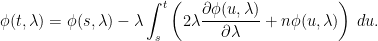
(2) implies (1): The idea is to derive a partial differential equation for the moment generating function of ${X_t}$ , and show that the solution is given by (4). Using the fact that ${X_t=M_t+nt}$ has quadratic variation ${[X]=4\int X_u\,du}$ , Ito’s lemma gives

$\displaystyle e^{-\lambda X_t}=e^{-\lambda X_s}+\int_s^te^{-\lambda X_u}\left(\frac12\lambda^24X_u-\lambda n\right)\,du -\lambda\int_s^t e^{-\lambda X_u}\,dM_u$

for constant ${\lambda\ge0}$ and times ${s\le t}$ . The final term is a local martingale and is bounded on finite time intervals (as all the other terms are). So, it is a proper martingale. Multiplying by a bounded ${\mathcal{F}_s}$ -measurable random variable Z and taking expectations,

$\displaystyle {\mathbb E}[Ze^{-\lambda X_t}]={\mathbb E}[Ze^{-\lambda X_s}]+\lambda\int_s^t{\mathbb E}[Ze^{-\lambda X_u}\left(2\lambda X_u-n)\right]\,du.$

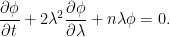
We now introduce the function ${\phi(t,\lambda)={\mathbb E}[Ze^{-\lambda X_t}]}$ and, noting that this has partial derivative ${\partial\phi/\partial\lambda=-{\mathbb E}[Ze^{-\lambda X_t}X_t]}$ ,

$\displaystyle \phi(t,\lambda)=\phi(s,\lambda)-\lambda\int_s^t\left(2\lambda\frac{\partial\phi(u,\lambda)}{\partial\lambda}+n\phi(u,\lambda)\right)\,du.$

So, ${\phi}$ is continuously differentiable over ${t\ge s}$ and, by differentiating the above equation, it satisfies the following partial differential equation

$\displaystyle \frac{\partial\phi}{\partial t}+2\lambda^2\frac{\partial\phi}{\partial\lambda}+n\lambda\phi=0.$

This is a transport equation and can be simplified by replacing ${\lambda}$ with a time dependent function ${\lambda_t}$ satisfying ${d\lambda_t/dt=2\lambda_t^2}$ ,

$\displaystyle \frac{d}{dt}\phi(t,\lambda_t)+n\lambda_t\phi(t,\lambda_t)=0.$

This is just an ordinary differential equation with the unique solution,

$\displaystyle \phi(t,\lambda_t)=e^{-n\int_s^t \lambda_u\,du}\phi(s,\lambda_s).$

(7)

The ODE for ${\lambda_t}$ is also easily solved, with the unique solution ${\lambda_s/(1-2\lambda_s (t-s))}$ . Using this, the following expressions can be calculated,

$\displaystyle \setlength\arraycolsep{2pt} \begin{array}{rl} &\displaystyle\lambda_s=\frac{\lambda_t}{1+2\lambda_t(t-s)},\smallskip\\ &\displaystyle e^{-n\int_s^t\lambda_u\,du}=\left(1+2\lambda_t(t-s)\right)^{-\frac{n}{2}}. \end{array}$

Substituting back into (7) and using ${\lambda=\lambda_t}$ gives equality (4) as required. ⬜

It is natural to ask about the properties of Bessel process paths such as, does it ever hit zero? Also, what happens to ${X_t}$ in the limit as t goes to infinity? We show below, in Theorem 7, that for ${n<2}$ the process hits zero at arbitrarily large times and, for ${n\ge2}$ it never hits zero. Furthermore, for ${n>2}$ it tends to infinity. The idea is to transform the process into a local martingale ${Y=f(X)}$ , so that standard convergence results for continuous local martingales can be applied. The function f is called the scale function of X.

Lemma 6 Let X be a ${{\rm BES}^2_n}$ process satisfying the SDE (6) with ${X_0>0}$ and make the following substitution.

If ${0<n<2}$ , let ${\tau}$ be the first time at which ${X_t=0}$ so that ${X^\tau}$ is the process stopped when it first hits zero, and set ${Y=(aX^\tau)^b}$ with

$\displaystyle b=1-\frac{n}{2},\ a=(2b)^{-2},\ c=1-\frac{1}{2b}=\frac{1-n}{2-n}.$ (8)

Then, Y satisfies the SDE

$\displaystyle dY=1_{\{Y>0\}}Y^c\,dW$ (9)

if ${n=2}$ then ${Y=\frac12\log X}$ satisfies

$\displaystyle dY=e^{-Y}\,dW$ (10)

if ${n>2}$ then ${Y=(aX)^b}$ with a, b, c as in (8) satisfies

$\displaystyle dY=-Y^c\,dW$ (11)

Although the substitutions above for ${n\ge2}$ are not defined when X=0, X remains strictly positive in this case.

Proof: For any ${n>0}$ , let ${\tau_n}$ be the first time at which ${X_t\le1/n}$ , so ${\tau_n\rightarrow\tau}$ and the stopped process ${X^{\tau_n}}$ is strictly positive. As ${f(x)=(ax)^b}$ is a smooth function on ${(0,\infty)}$ , Ito’s lemma can be applied to ${Y=f(X)}$ on the interval ${[0,\tau_n]}$ ,

$\displaystyle \setlength\arraycolsep{2pt} \begin{array}{rl} \displaystyle dY_t&\displaystyle=a^bbX_t^{b-1}\left(2\sqrt{X_t}\,dW_t+n\,dt\right)+\frac12a^bb(b-1)X_t^{b-2}\,d[X]_t\smallskip\\ &\displaystyle=2a^bbX_t^{b-1/2}\,dW_t+2a^bb\left(n/2+b-1\right)X_t^{b-1}\,dt. \end{array}$

Here, the expression ${d[X]=4X\,dt}$ has been used. If ${n\not=2}$ then substituting expression (8) for b makes the last term on the right hand side equal to zero. So,

$\displaystyle \setlength\arraycolsep{2pt} \begin{array}{rl} \displaystyle dY&\displaystyle=2a^bb\left(Y^{1/b}/a\right)^{b-1/2}\,dW\smallskip\\ &\displaystyle=2a^{1/2}bY^c\,dW. \end{array}$

Using ${a^{1/2}=\vert 2b\vert^{-1}}$ gives ${2a^{1/2}b=\pm1}$ according to whether b is positive ( ${n<2}$ ) or negative ( ${n>2}$ ). So,

$\displaystyle dY=\pm Y^c\,dW$

on the interval ${[0,\tau_n]}$ . Letting n increase to infinity, we see that equations (9) and (11) are satisfied on the interval ${[0,\tau)}$ . If ${n<2}$ then ${b>0}$ , so ${Y=(aX^\tau)^b}$ is equal to zero over the interval ${[\tau,\infty)}$ , and (9) is satisfied. On the other hand, if ${n>2}$ then ${b<0}$ so Y explodes to infinity at time ${\tau}$ . However, ${Y^{\tau_n}}$ is a nonnegative local martingale and cannot explode in a finite time. This is a consequence of Fatou’s lemma,

$\displaystyle {\mathbb E}[\liminf_{n\rightarrow\infty}Y_{\tau_n}\mid\mathcal{F}_0]\le\liminf_{n\rightarrow\infty}{\mathbb E}[Y_{\tau_n}\mid\mathcal{F}_0]\le Y_0.$

So, Y is almost surely bounded and ${\tau=\infty}$ .

Now, consider the case with ${n=2}$ and ${Y=\frac12\log(X)}$ . As ${f(x)=\frac12\log(x)}$ is smooth on ${(0,\infty)}$ , Ito’s lemma can be applied on the interval ${[0,\tau_n]}$ , in a similar way as above,

$\displaystyle \setlength\arraycolsep{2pt} \begin{array}{rl} \displaystyle dY_t&\displaystyle=\frac{1}{2X_t}\left(2\sqrt{X_t}\,dW_t+2\,dt\right)-\frac{1}{4X_t^2}\,d[X]_t\smallskip\\ &\displaystyle=X_t^{-1/2}\,dW_t\smallskip\\ &\displaystyle=e^{-Y_t}\,dW_t. \end{array}$

As above, this holds over the interval ${[0,\tau)}$ and it needs to be shown that ${\tau=\infty}$ almost surely. Letting ${\sigma}$ be the first time at which ${X\ge K}$ for some constant K, Y is a local martingale bounded above over the interval ${[0,\sigma)}$ . Applying Fatou’s lemma to –Y,

$\displaystyle {\mathbb E}[\limsup_{n\rightarrow\infty}Y_{\sigma\wedge\tau_n}\mid\mathcal{F}_0]\ge\limsup_{n\rightarrow\infty}{\mathbb E}[Y_{\sigma\wedge\tau_n}\mid\mathcal{F}_0]\ge Y_0.$

However ${Y=\frac12\log(X)}$ diverges to ${-\infty}$ at time ${\tau}$ , so ${\tau_n>\sigma}$ for large enough n (almost surely). Letting K increase to infinity, ${\sigma}$ goes to infinity, showing that ${\tau=\lim_n\tau_n}$ is almost surely infinite, as required. ⬜

Using the transformation given by Lemma 6 together with the convergence of continuous local martingales, it is possible to say whether a ${{\rm BES}^2_n}$ process hits zero and to determine ${\liminf_tX_t}$ and ${\limsup_tX_t}$ , for each value of n.

Theorem 7 Let X be a ${{\rm BES}^2_n}$ process. With probability one,

if ${n=0}$ then X hits 0 at some time, and remains there.

if ${0<n<2}$ then X hits zero at arbitrarily large times and ${\limsup_{t\rightarrow\infty}X_t=\infty}$ .

if ${n=2}$ then X is strictly positive at all positive times and ${\liminf_{t\rightarrow\infty}X_t=0}$ , ${\limsup_{t\rightarrow\infty}X_t=\infty}$ .

if ${n>2}$ then X is strictly positive at all positive times and ${X_t\rightarrow\infty}$ as ${t\rightarrow\infty}$ .

Recall that the convergence theorem for continuous local martingales states that the events on which a continuous local martingale Y converges to a finite limit, the event on which ${\liminf_{t\rightarrow\infty}Y_t\not=-\infty}$ , and on which ${\limsup_{t\rightarrow\infty}Y_t\not=\infty}$ , are all identical (up to zero probability sets). This fact is used several times in the following proof.

Proof: The case with ${n=0}$ is easy. We have already shown that it hits zero with probability ${\exp(-X_0/(2t))}$ by time t conditional on ${\mathcal{F}_0}$ and that, once it hits zero, it stays there. Letting t increase to infinity this converges to 1, so it hits zero almost surely at some positive time.

Let us show that ${\limsup_tX_t=\infty}$ for all ${n>0}$ . From the definition, ${X_t/t}$ has the ${\chi^2_n(X_0/t)}$ distribution conditional on ${\mathcal{F}_0}$ , which can be written as the sum of independent random variables ${U\sim\chi^2_n(0)}$ and ${V\sim\chi^2_0(X_0/t)}$ . So, for any constant ${K\ge0}$ ,

$\displaystyle \setlength\arraycolsep{2pt} \begin{array}{rl} \displaystyle{\mathbb P}(X_t>K)&\displaystyle={\mathbb P}(U+V>K/t)\ge{\mathbb P}(U>K/t)\smallskip\\ &\displaystyle\rightarrow{\mathbb P}(U>0)=1. \end{array}$

as ${t\rightarrow\infty}$ , so ${\limsup_{t\rightarrow\infty}X_t=\infty}$ .

For ${n\ge2}$ it was shown in Lemma 6 that X never hits 0 at any time conditional on ${X_0>0}$ . As it has zero probability of being equal to zero at a time ${t>0}$ , this shows that it never hits zero on ${[t,\infty)}$ and, letting t decrease to zero, it never hits zero at any positive time.

Now, consider ${0<n<2}$ . As shown in Lemma 6, ${Y=f(X^\tau)}$ is a nonnegative local martingale for some continuous and strictly increasing function satisfying ${f(0)=0}$ , where ${X^\tau}$ is the process stopped when it first hits zero. As this trivially satisfies ${\liminf_tY_t\not=-\infty}$ , martingale convergence implies that ${Y_\infty=\lim_tY_t}$ exists and is finite almost surely. However, as we have just shown, ${\limsup_tX_t}$ is infinite, so ${Y\not=f(X)}$ at large enough times. This can only happen if the process hits zero, after which Y is stopped at zero.

Alternatively, if ${n=2}$ , then ${Y=f(X)}$ is a local martingale for ${f(x)=\log(x)/2}$ . As shown above, ${\limsup_tY_t}$ is infinite so, by martingale convergence, ${\liminf_tY_t=-\infty}$ . Therefore, ${\liminf_tX_t=0}$ .

Finally, it only remains to show that ${X_t\rightarrow\infty}$ for ${n>2}$ . Again, using Lemma 6, ${Y=f(X)}$ is a nonnegative local martingale for a strictly positive and continuous function f satisfying ${f(x)\rightarrow0}$ as ${x\rightarrow\infty}$ . As above, martingale convergence implies that ${Y_\infty=\lim_tY_t}$ exists almost surely. However, since we have already shown that ${\limsup_tX_t=\infty}$ , it follows that ${Y_\infty=\liminf_tY_t=0}$ . So, ${f(X_t)\rightarrow0}$ as ${t\rightarrow\infty}$ , giving ${X_t\rightarrow\infty}$ as required. ⬜

An immediate consequence of the preceding result is to n-dimensional standard Brownian motion. For positive integers n, the squared Bessel process was introduced above as the squared magnitude ${\Vert B\Vert^2}$ of an n-dimensional Brownian motion. In one and two dimensions, we see that Brownian motion is recurrent. That is, with probability one, it enters every nonempty set ${U\subseteq{\mathbb R}^n}$ at arbitrarily large times. As ${{\mathbb R}^n}$ has a countable base for the topology, it is enough to prove this for a countable collection of open sets and, by countable additivity of probability measures, it is equivalent to saying that X almost surely enters the open set U at arbitrarily large times, for each open ${U\not=\emptyset}$ individually.

In three or more dimensions, Brownian motion is not recurrent. In fact, it diverges to infinity with probability one.

Theorem 8 Let B be an n-dimensional Brownian motion. With probability one,

if ${n\le2}$ then B is recurrent.

if ${n\ge3}$ then ${\Vert B_t\Vert\rightarrow\infty}$ as ${t\rightarrow\infty}$ .

Proof: For ${n\le2}$ , let ${U\subseteq{\mathbb R}^n}$ be a nonempty open set and choose ${x\in U}$ . Then, ${X\equiv\Vert B-x\Vert^2}$ is a ${{\rm BES}^2_n}$ process. By Theorem 7, ${\liminf_tX_t=0}$ , so ${X_t\in U}$ at arbitrarily large times.

If ${n\ge3}$ then ${X\equiv\Vert B\Vert^2}$ is a ${{\rm BES}^2_n}$ process so, by Theorem 7, ${X_t\rightarrow\infty}$ as ${t\rightarrow\infty}$ . ⬜

Finally for this post, I show that Bessel process are well defined Markov processes and that continuous modifications do indeed exist.

Lemma 9 Fix any ${n\ge0}$ and, for each ${t\ge0}$ , let ${P_t}$ be the transition probability on ${{\mathbb R}_+}$ such that, for each ${x\in{\mathbb R}_+}$ , ${P_t(x,\cdot)}$ has moment generating function given by

$\displaystyle \int e^{-\lambda y}\,P_t(x,dy)=\left(1+2\lambda t\right)^{-\frac{n}{2}}\exp\left(\frac{-\lambda x}{1+2\lambda t}\right).$ (12)

Then, ${\{P_t\}_{t\ge0}}$ is a Feller transition function. Furthermore, any Markov process with this transition function has a continuous modification, which is then a ${{\rm BES}^2_n}$ process.

Proof: To show that ${\{P_t\}}$ is a transition function, it is only necessary to prove the Chapman-Kolmogorov equation ${P_sP_t=P_{s+t}}$ . This can be verified by directly computing the moment generating functions. Setting ${\lambda^\prime=\lambda/(1+2\lambda t)}$ ,

$\displaystyle \setlength\arraycolsep{2pt} \begin{array}{rl} \displaystyle\int\!\!\int e^{-\lambda z}\,P_t(y,dz)P_s(x,dy)&\displaystyle=(1+2\lambda t)^{-\frac{n}{2}}\int e^{-\lambda^\prime y}\,P_s(x,dy)\smallskip\\ &\displaystyle=(1+2\lambda t)^{-\frac{n}{2}}(1+2\lambda^\prime s)^{-\frac{n}{2}}\exp\left(\frac{-\lambda^\prime x}{1+2\lambda^\prime s}\right)\smallskip\\ &\displaystyle=(1+2\lambda(s+t))^{-\frac{n}{2}}\exp\left(\frac{-\lambda x}{1+2\lambda(s+t)}\right)\smallskip\\ &\displaystyle=\int e^{-\lambda y}\,P_{s+t}(x,dy), \end{array}$

so ${P_sP_t=P_{s+t}}$ as required.

We now move on to the proof that this is a Feller transition function. It needs to be shown that for any ${f\colon{\mathbb R}_+\rightarrow{\mathbb R}}$ in the set ${C_0=C_0({\mathbb R}_+)}$ of continuous functions vanishing at infinity, then ${P_tf\in C_0}$ and ${P_tf(x)\rightarrow f(x)}$ as ${t\rightarrow 0}$ . First, if ${f(x)=e^{-\lambda x}}$ for a constant ${\lambda>0}$ then

$\displaystyle P_tf(x)=(1+2\lambda t)^{-n/2}\exp(-\lambda x/(1+2\lambda t)),$

which satisfies the required properties. This extends to all ${f\in C_0(E)}$ by uniformly approximating by linear combinations of such functions (see Lemma 10 below).

It only remains to show that a Markov process X with the transition function ${\{P_t\}}$ has a continuous modification. Any such process automatically satisfies (4) and, if it is continuous, is a squared Bessel process by definition. By the existence of cadlag modifications for Feller processes, we may assume that X is cadlag. It just needs to be shown that the jumps ${\Delta X_t=X_t-X_{t-}}$ are almost surely equal to zero. If ${s_n<t\le t_n}$ are a sequence of times with ${t_n-s_n\rightarrow0}$ , then ${X_{t_n}-X_{s_n}\rightarrow\Delta X_t}$ . From this, the following inequality is obtained, bounding the maximum jump of X over the interval ${[0,t]}$ .

$\displaystyle \liminf_{n\rightarrow\infty}\sum_{k=1}^n(X_{kt/n}-X_{(k-1)t/n})^4\ge\max_{s\le t}(\Delta X_s)^4.$

(13)

We show that the left hand side converges to zero in probability. The moment generating function of ${X_t-X_s}$ can be computed from (4),

$\displaystyle \setlength\arraycolsep{2pt} \begin{array}{rl} &\displaystyle{\mathbb E}\left[\exp\left(-\lambda(X_t-X_s)\right)\;\middle\vert\;\mathcal{F}_0\right]\smallskip\\ &\displaystyle=\left(1+2\lambda(t-s)\right)^{-\frac{n}{2}}{\mathbb E}\left[\exp\left(\frac{-\lambda X_s}{1+2\lambda(t-s)}+\lambda X_s\right)\;\middle\vert\;\mathcal{F}_0\right]\smallskip\\ &\displaystyle=\left(1+2\lambda(t-s)\right)^{-\frac{n}{2}}\left(1-2\lambda^\prime s\right)^{-\frac{n}{2}}\exp\left(\frac{\lambda^\prime X_0}{1-2\lambda^\prime s}\right). \end{array}$

where ${\lambda^\prime=2\lambda^2(t-s)/(1+2\lambda(t-s))}$ . The expected value of ${(X_t-X_s)^4}$ conditional on ${\mathcal{F}_0}$ can be calculated by expanding this out as a power series and looking at the coefficient of ${\lambda^4}$ . This is a bit messy but, noting that the expression above expands in terms of ${\lambda(t-s)}$ and ${\lambda^2(t-s)}$ , we see that the coefficient of ${\lambda^4}$ will be equal to ${(t-s)^2}$ multiplied by a polynomial in t–s, s and ${X_0}$ . Therefore,

$\displaystyle {\mathbb E}[(X_t-X_s)^4\mid\mathcal{F}_0]=O((t-s)^2)$

over any bounded range for s and t. Taking the expected value conditional on ${\mathcal{F}_0}$ , it follows that the left hand side of (13) goes to zero at rate ${n^{-1}}$ . So, ${\max_{s\le t}(\Delta X_s)^4}$ is almost surely zero, as required. ⬜

The following result for uniformly approximating continuous functions on ${{\mathbb R}_+}$ was used in the proof that ${P_t}$ is a Feller transition function.

Lemma 10 The set of linear combinations of functions of the form ${x\mapsto e^{-\lambda x}}$ for ${\lambda>0}$ is dense in ${C_0({\mathbb R}_+)}$ (in the uniform norm).

Proof: Any ${f\in C_0({\mathbb R}_+)}$ can be written as ${f(x)=g(e^{-x})}$ where ${g\colon[0,1]\rightarrow{\mathbb R}}$ is continuous with ${g(0)=0}$ . By the Stone-Weierstrass approximation theorem there are polynomials ${p_n}$ converging uniformly to g on the unit interval. Replacing ${p_n}$ by ${p_n-p_n(0)}$ if necessary, we can suppose that ${p_n(0)=0}$ . Then, ${p_n(e^{-x})}$ are linear combinations of functions of the form ${e^{-kx}}$ for ${k>0}$ and ${p_n(e^{-x})}$ converges uniformly to ${f(x)}$ . ⬜

11 thoughts on “Bessel Processes”

Alekk says:

28 July 10 at 2:56 PM

Dear George,

how would you (efficiently) simulate a BES^2_n process in such a manner that the process does stay positive (for non integer dimension n, indeed).

thanks again for these great posts!
Best
PS: tiny typo in the definition of $Y$ in equation (8)

1. George Lowther says:
  
  29 July 10 at 2:17 AM
  
  Hi. I can give a quick answer now, but I’m not going to have much time to go into details for a few days.
  
  1) You can sample a Bessel process exactly at a fixed sequence of times, by sampling from the skew chi-square distributions. As I explained near the top of the post, a $\chi^2_n(\mu)$ distribution can be written as $X=Y+\sum_{i=1}^{2N}Z_i^2$ where, Y is $\chi^2_n$ , Z_i are standard normal and N is Poisson of rate $\mu/2$ . Equivalently, $Y\sim\chi^2_{n+2N}$ conditional on N. See the paper Exact Simulation of Bessel Diffusions which includes this and other related methods (actually, I found that paper while searching for another one which I remember from several years ago but forget the title. I’ll come back with the link if I remember…)
  
  2) You can numerically simulate the SDE (3), which only gives an approximate solution, but will likely be much faster if you want to sample it at a dense set of times. It can be done by an Euler scheme. However, if the process is close to zero then the simulation could jump below zero. Then you would have to max with zero, which would bias the distribution causing the drift to increase as the process gets close to zero. This would cause the approximation to converge very slowly in the number of time steps used when n is small. A better way would be to modify the Euler scheme so that you are sampling positive numbers from the start while matching all the moments of dX up to O(dt^k), some appropriate k. For example, a trinomial distribution could be used to match all moments up to O(dt³), leading to an O(dt²) error term overall.
  
2. George Lowther says:
  
  29 July 10 at 2:32 AM
  
  and, what’s the typo?
  
Alekk says:

31 July 10 at 4:12 AM

thank you for these very interesting answer, and the reference !

I remember a discussion where someone advised me to take the scale function $f$ of a diffusion $X_t$ and to try to simulate $Y_t=f(X_t)$ : this would often eliminate the problem of staying positive (boundary effect), say, and would often be much more precise: I do not remember really well the motivation for that, though. From a practical point of view, why $f(x) = \log(x)$ would be worse than taking the scale function in this problem, for example. In one case $Y_t=f(X_t)$ is obviously a martingale, but I do not understand why this is better. Could you shed some light on this issue ?

Thank you for this fantastic blog!
PS: tiny typo in the definition of $Y$ above eq 8, no ?

1. George Lowther says:
  
  7 August 10 at 3:42 AM
  
  I’m not sure why applying the scale function should eliminate any boundary effect. If you have a squared Bessel process of dimension n < 2, then the scale function is a positive power of X (Lemma 5 above). So it still has a boundary at zero. Also, if n=2, then the scale function is log(x). This does remove the boundary, but the SDE for Y=log(X) is dY = e^-Y dW which has exponentially growing coefficients as Y goes negative. That does not look very promising from the point of view of obtaining accurate simulations.
  
  In general, whether or not transforming by the scale function improves the simulations must depend on what particular SDE you start with and what simulation method you are using.
  
  Another point: if f is the scale function then Y=f(X) does not have to be a martingale. In fact, for squared Bessel processes of dimension n > 0, this is never the case. For n < 2 it has a reflecting boundary, so only becomes a martingale if you stop the process at the boundary. For n>=2 the boundary is never attained but, still, Y is not a martingale. It’s just a local martingale.
  
  [Apols. for not responding sooner. Not had chance to log on to my machine the last week].
  
2. George Lowther says:
  
  7 August 10 at 3:48 AM
  
  Also, thanks for mentioning that the transformation I use in Lemma 5 is called the scale function. I updated the text to mention this.
  
  Still don’t see the typo. I have Y = (aX^τ)^b, which is what was intended. Maybe you are thinking that a should be outside the parentheses? But, that’s not true with my definition of a.
  
Alekk says:

14 August 10 at 6:48 PM

Thank you for all these very interesting comments (and apologize for this very late answer): seems like I have been a little bit optimistic with this “scale function” transformation!

Btw, numerical simulations of SDEs seem to be a very broad area: do you plan on writing on this ?

1. George Lowther says:
  
  15 August 10 at 11:49 PM
  
  I don’t have any immediate plans to post about numerical simulations. Maybe, at some point. I’ll bear your suggestion in mind though.
  
g says:

15 May 12 at 10:35 PM

Hi George,

Great blog btw, really helpful and concise in clarifying many important concepts of stochastic processes. Just wanted to point out a small typo in Theorem 4 (3) -> (2): I think you want $X_t - nt = 2 \int_0^t \sqrt{X_s} dW_s$ .

1. George Lowther says:
  
  29 October 19 at 8:45 PM
  
  Thanks! I eventually fixed this typo!
  
Pingback: References on the (reflected) Bessel process: construction, formulas, densities, properties – Mathematics – Forum

	Harry on Filtrations and Adapted P…
	Anonymous on Analytic Sets
	Daniel on Analytic Sets
	Sid on Martingale Convergence
	northwiz on Preservation of the Local Mart…
	George Lowther on Martingale Convergence
	Sid on Martingale Convergence
	George Lowther on The Burkholder-Davis-Gundy Ine…
	George Lowther on Preservation of the Local Mart…
	northwiz on Preservation of the Local Mart…

Bessel Processes

Published by George Lowther

11 thoughts on “Bessel Processes”

Leave a Reply Cancel reply

Like this:

Related

Published by George Lowther

11 thoughts on “Bessel Processes”

Leave a Reply Cancel reply