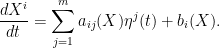
Existence of Solutions to Stochastic Differential Equations

A stochastic differential equation, or SDE for short, is a differential equation driven by one or more stochastic processes. For example, in physics, a Langevin equation describing the motion of a point ${X=(X^1,\ldots,X^n)}$ in n-dimensional phase space is of the form

$\displaystyle \frac{dX^i}{dt} = \sum_{j=1}^m a_{ij}(X)\eta^j(t) + b_i(X).$

(1)

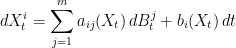
The dynamics are described by the functions ${a_{ij},b_i\colon{\mathbb R}^n\rightarrow{\mathbb R}}$ , and the problem is to find a solution for X, given its value at an initial time. What distinguishes this from an ordinary differential equation are random noise terms ${\eta^j}$ and, consequently, solutions to the Langevin equation are stochastic processes. It is difficult to say exactly how ${\eta^j}$ should be defined directly, but we can suppose that their integrals ${B^j_t=\int_0^t\eta^j(s)\,ds}$ are continuous with independent and identically distributed increments. A candidate for such a process is standard Brownian motion and, up to constant scaling factor and drift term, it can be shown that this is the only possibility. However, Brownian motion is nowhere differentiable, so the original noise terms ${\eta^j=dB^j_t/dt}$ do not have well defined values. Instead, we can rewrite equation (1) is terms of the Brownian motions. This gives the following SDE for an n-dimensional process ${X=(X^1,\ldots,X^n)}$

$\displaystyle dX^i_t = \sum_{j=1}^m a_{ij}(X_t)\,dB^j_t + b_i(X_t)\,dt$

(2)

where ${B^1,\ldots,B^m}$ are independent Brownian motions. This is to be understood in terms of the differential notation for stochastic integration. It is known that if the functions ${a_{ij}, b_i}$ are Lipschitz continuous then, given any starting value for X, equation (2) has a unique solution. In this post, I give a proof of this using the basic properties of stochastic integration as introduced over the past few posts.

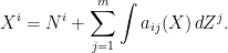
First, in keeping with these notes, equation (2) can be generalized by replacing the Brownian motions ${B^j}$ and time t by arbitrary semimartingales. As always, we work with respect to a complete filtered probability space ${(\Omega,\mathcal{F},\{\mathcal{F}_t\}_{t\ge 0},{\mathbb P})}$ . In integral form, the general SDE for a cadlag adapted process ${X=(X^1,\ldots,X^n)}$ is as follows,

$\displaystyle X^i = N^i + \sum_{j=1}^m\int a_{ij}(X)\,dZ^j.$

(3)

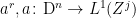
Here, ${Z^1,\ldots,Z^m}$ are semimartingales. For example, as well as Brownian motion, Lévy processes are often also used. If ${N^i}$ are ${\mathcal{F}_0}$ -measurable random variables, they simply specify the starting value ${X_0=N}$ . More generally, in (3), we can allow N to be any cadlag and adapted process, which acts as a `source term’ in the SDE. Furthermore, rather than just being functions of X at time t, we allow ${a_{ij}(X)_t}$ to be a function of the process X at all times up to t. For example, it could depend on it maximum so far, or a running average. In that case, we instead impose a functional Lipschitz condition as follows. The notation ${X^*_t\equiv\sup_{s\le t}\Vert X_s\Vert}$ is used for the maximum of a process X, and ${{\rm D}^n}$ denotes the set of all cadlag and adapted n-dimensional processes.

(P1) ${X\mapsto a_{ij}(X)}$ is a map from ${{\rm D}^n}$ to the set ${L^1(Z^j)}$ of predictable and ${Z^j}$ –integrable processes.
(P2) There is a constant K such that

$\displaystyle \vert a_{ij}(X)_t-a_{ij}(Y)_t\vert \le K(X-Y)^*_{t-}$

for all times ${t>0}$ and ${X,Y\in{\rm D}^n}$ .

The special case where ${a_{ij}(X)_t}$ is a Lipschitz continuous function of ${X_{t-}}$ clearly satisfies both (P1) and (P2). The uniqueness theorem for SDEs with Lipschitz continuous coefficients is as follows.

Theorem 1 Suppose that ${a_{ij}}$ satisfy properties (P1), (P2). Then, there is a unique ${X\in{\rm D}^n}$ satisfying SDE (3).

Recall that, throughout these notes, we are identifying any processes which agree on a set of probability one so that, here, uniqueness refers to uniqueness up to evanescence.

Simple examples of SDEs with Lipschitz coefficients include linear equations such as mean reverting Ornstein-Uhlenbeck processes, geometric Brownian motion and Doléans exponentials.

After existence and uniqueness, an important property of solutions to SDEs is stability. That is, small changes to the coefficients only have a small effect on the solution. The notion of a `small change’ first needs to be made precise by specifying a topology on these terms. For the coefficients ${a_{ij}}$ , uniform convergence on bounded sets will be used. Given maps ${a^r,a\colon{\rm D}^n\rightarrow L^1(Z^j)}$ for r=1,2,…, I will say that ${a^r\rightarrow a}$ uniformly on bounded sets if, for each ${t,L>0}$

$\displaystyle \sup\left\{\vert a^r(X)_s-a(X)_s\vert\colon s\le t, X\in{\rm D}^n, X^*_{t-}\le L\right\}$

tends to zero as r goes to infinity. For the solutions X and source term N, which are cadlag processes, the appropriate topology is that of convergence uniformly on compacts in probability (ucp convergence). Recall that ${X^r\xrightarrow{\rm ucp}X}$ if ${(X^r-X)^*_t\rightarrow 0}$ in probability for each t. The stability of solutions to SDEs under small changes to the coefficients can then be stated precisely.

Theorem 2 Suppose that ${a_{ij}}$ satisfy properties (P1), (P2) and let X be the unique solution to the SDE (3) given by Theorem 1. Suppose furthermore that ${M^r\in{\rm D}^n}$ and ${a^r_{ij}\colon{\rm D}^n\rightarrow L^1(Z^j)}$ are sequences such that ${M^r\xrightarrow{\rm ucp}N}$ and ${a^r_{ij}\rightarrow a_{ij}}$ uniformly on bounded sets. Then, any sequence of processes ${X^r\in{\rm D}^n}$ satisfying

$\displaystyle (X^r)^i = (M^r)^i+\sum_{j=1}^m\int a^r_{ij}(X^r)\,dZ^j$

converges ucp to X as r goes to infinity.

Equivalently, the map from ${(N,a_{ij})}$ to the solution X satisfying SDE (3) is continuous under the respective topologies.

Proof of Existence and Uniqueness

Throughout this subsection, assume that N is a cadlag adapted n-dimensional process, ${Z^j}$ are semimartingales and that ${a_{ij}}$ satisfy properties (P1), (P2) above. To simplify the notation a bit, for any ${X\in{\rm D}^n}$ , write ${F(X)=(F(X)^1,\ldots,F(X)^n)}$ to denote the following n-dimensional process,

$\displaystyle F(X)^i=N^i+\sum_{j=1}^n\int a_{ij}(X)\,dZ^j.$

So, ${F\colon{\rm D}^n\rightarrow{\rm D}^n}$ and equation (3) just says that X=F(X). Existence and uniqueness of solutions to this SDE is equivalent to F having a unique fixed point.

The `standard’ proof for Lipschitz continuous coefficients, at least when the driving semimartingales are Brownian motions, makes use of the Ito isometry to construct a norm on the cadlag processes under which F is a contraction. The result then follows from the contraction mapping theorem. Although this method can also be applied for arbitrary semimartingales, it is more difficult and some rather advanced results on semimartingale decompositions are required. However, the aim here is to show how existence and uniqueness follows for all semimartingales as a consequence of the basic properties of the stochastic integration, so a different approach is taken. Furthermore, the method used of constructing discrete approximations making the error term X-F(X) small is closer to methods which might be employed in practice when explicitly simulating solutions to (3).

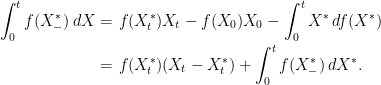
First, the following inequality bounds the values of a positive semimartingale X in terms of the maximum value of the stochastic integral ${\int(1/X^*_-)\,dX}$ .

Lemma 3 Let X be a positive semimartingale. Then,

$\displaystyle \left(\int\frac{1}{X^*_-}\,dX\right)^*\ge\log(X^*/X_0).$

Proof: For any continuous decreasing function ${f}$ , ${f(X^*)}$ is a cadlag decreasing process and integration by parts gives the following,

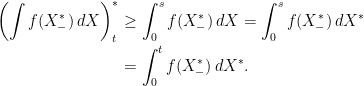
$\displaystyle \int f(X^*_-)\,dX = f(X^*)X - f(X_0)X_0 - \int X\,df(X^*).$

It is easily seen that ${X^*_-}$ is constant over any interval ${[s,t)}$ on which ${X\not=X^*}$ and, therefore, the integral above with respect to ${f(X^*)}$ is zero over such intervals. So, we can replace the integrand ${X}$ by ${X^*}$ and, again applying integration by parts,

$\displaystyle \setlength\arraycolsep{2pt} \begin{array}{rl} \displaystyle\int_0^t f(X^*_-)\,dX =&\displaystyle f(X^*_t)X_t - f(X_0)X_0 - \int_0^t X^*\,df(X^*)\smallskip\\ \displaystyle=&\displaystyle f(X^*_t)(X_t-X^*_t) + \int_0^t f(X^*_-)\,dX^*. \end{array}$

(4)

As the process is cadlag, there must exist an ${s\le t}$ such that either ${X_s=X^*_t}$ or ${X_{s-}=X^*_t}$ . In the first case, evaluating (4) at time s gives

$\displaystyle \setlength\arraycolsep{2pt} \begin{array}{rl} \displaystyle\left(\int f(X^*_-)\,dX\right)^*_t&\displaystyle\ge\int_0^s f(X^*_-)\,dX = \int_0^s f(X^*_-)\,dX^*\smallskip\\ &\displaystyle=\int_0^t f(X^*_-)\,dX^*. \end{array}$

The final equality follows from the fact that ${X^*}$ must be constant on the interval [s,t]. Similarly, in the case where ${X_{s-}=X^*_t}$ , the same inequality results from evaluating (4) at time s-.

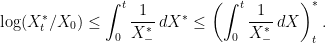
We are only interested in the special case ${f(x)=1/x}$ . The next step is to apply the generalized Ito formula to ${\log(X^*)}$ .

$\displaystyle \log(X^*_t/X_0) = \int_0^t\frac{1}{X^*}\,dX^* + \sum_{s\le t}\left(\Delta\log(X^*_s)-\frac{1}{X^*_{s-}}\Delta X^*_s\right).$

The inequality ${\log(1+x)-x\le 0}$ follows from concavity of the logarithm and, putting ${x=\Delta X^*_s/X^*_{s-}}$ shows that the summation above is non-positive,

$\displaystyle \log(X^*_t/X_0)\le\int_0^t\frac{1}{X^*_-}\,dX^*\le\left(\int_0^t\frac{1}{X^*_-}\,dX\right)^*_t.$

⬜

The general idea behind the proofs given here is that if X,Y are processes such that the error terms X-F(X) and Y-F(Y) to the SDE (3) are small then

$\displaystyle X-Y\approx F(X)-F(Y)=\sum_{j=1}^m\int (a_{ij}(X)-a_{ij}(Y))\,dZ^j.$

The Lipschitz property implies that the integrand ${a_{ij}(X)-a_{ij}(Y)}$ is bounded by ${K(X-Y)^*_-}$ , and the following result will be used to show that ${X\approx Y}$ .

Lemma 4 Let ${X^r=(X^{r,1},\ldots,X^{r,n})}$ be a sequence of n-dimensional processes satisfying

$\displaystyle X^{r,i}=\sum_{j=1}^m\int\alpha^r_{ij}\,dZ^j+N^{r,i}$

for predictable processes ${\vert\alpha^r_{ij}\vert\le K{X^r}^*_-}$ and cadlag adapted processes ${N^r}$ converging ucp to zero as r goes to infinity. Then, ${X^r\xrightarrow{\rm ucp}0}$ .

Proof: By definition of ucp convergence, for any ${\epsilon>0}$ the limit ${{\mathbb P}( {N^r}^*_t\ge \epsilon)\rightarrow 0}$ holds as r goes to infinity. Therefore, there exists a sequence ${\epsilon_r\downarrow 0}$ such that ${{\mathbb P}({N^r}_t^*\ge\epsilon_r)\rightarrow 0}$ . So, by stopping the processes as soon as ${\Vert N^r\Vert\ge\epsilon_r}$ , we may assume that ${\Vert N^r\Vert\le\epsilon_r}$ for all r.

Now, writing ${Y^r\equiv X^r - N^r}$ ,

$\displaystyle Y^{r,i} = \sum_{j=1}^m\int ( {Y^r}^*_- + \epsilon_r)\beta^r_{ij}\,dZ^j$

for predictable processes ${\beta^r_{ij}=\alpha^r_{ij}/{({Y^r}^*_-+\epsilon_r)}}$ , which are uniformly bounded by K. Applying Lemma 3 to the nonnegative semimartingale ${\Vert Y^r\Vert^2+\epsilon_r^2}$ ,

$\displaystyle \log\left(\epsilon_r^{-2}({Y^r}^*)^2+1\right)\le\left(\int \frac{d\Vert Y^r\Vert^2}{({Y^r}^*_-)^2+\epsilon_r^2}\right)^*.$

However, applying integration by parts to ${\Vert Y^r\Vert^2=\sum_i(Y^{r,i})^2}$ ,

$\displaystyle \setlength\arraycolsep{2pt} \begin{array}{l} \displaystyle\int \frac{d\Vert Y^r\Vert^2}{({Y^r}^*_-)^2+\epsilon_r^2}= \sum_i\left(2\int \frac{Y^{r,i}_-\,dY^{r,i}}{({Y^r}^*_-)^2+\epsilon_r^2}+\int\frac{d[Y^{r,i}]}{({Y^r}^*_-)^2+\epsilon_r^2}\right)\smallskip\\ \displaystyle= \sum_{i,j}\left(2\int \frac{Y^{r,i}_-({Y^r}^*_-+\epsilon_r)}{({Y^r}^*_-)^2+\epsilon_r^2}\beta^r_{ij}\,dZ^j+\int\frac{({Y^r}^*_-+\epsilon_r)^2}{({Y^r}^*_-)^2+\epsilon_r^2}(\beta^r_{ij})^2\,d[Z^j]\right) \end{array}$

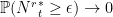
The inequality ${(y+\epsilon)^2\le 2(y^2+\epsilon^2)}$ shows that the integrands on the right hand side of the above expression are all bounded by ${\sqrt{2}K}$ in the first integral and by ${2K^2}$ in the second integral. Hence, by dominated convergence, if ${\lambda_r\rightarrow 0}$ is a sequence of real numbers then

$\displaystyle \lambda_r\log(\epsilon_r^{-2}({Y^r}^*)^2+1)\le\left(\lambda_r\int\frac{d\Vert Y^r\Vert^2}{({Y^r}^*_-)^2+\epsilon_r^2}\right)^*\rightarrow 0$

in probability as ${r\rightarrow\infty}$ . This shows that the sequence ${\log(\epsilon_r^{-2}({Y^r}^*)^2+1)}$ is bounded in probability as ${r\rightarrow\infty}$ and, by exponentiating, ${\epsilon_r^{-1}{Y^r}^*_t}$ is bounded in probability. However, ${\epsilon_r^{-1}\rightarrow\infty}$ and therefore, ${Y^r\xrightarrow{\rm ucp} 0}$ . Finally, ${X^r=Y^r+N^r\xrightarrow{\rm ucp} 0}$ as required. ⬜

Now, with the aid of the previous result, it is possible to construct approximate solutions to the SDE (3) making the error X-F(X) as small as we like.

Lemma 5 For any ${\epsilon>0}$ there exists an ${X\in{\rm D}^n}$ satisfying ${\Vert X-F(X)\Vert<\epsilon}$ .

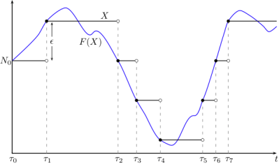
Figure 1: Approximate solution to the SDE X=F(X)

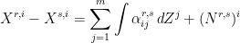
Proof: The idea is to define X inductively as a piecewise constant function across finite time intervals, while adjusting the time step sizes to force the error to remain within the tolerance ${\epsilon}$ . To do this, define stopping times ${\tau_r}$ and processes ${X^{(r)}}$ by ${\tau_0=0, X^0=N_0}$ and, for ${r\ge 0}$ ,

$\displaystyle \setlength\arraycolsep{2pt} \begin{array}{l} \displaystyle X^{(r+1)}_t=\begin{cases} X^{(r)}_t,&\textrm{if }t<\tau_r,\\ F(X^{(r)})_{\tau_r},&\textrm{if }t\ge\tau_r, \end{cases}\smallskip\\ \displaystyle\tau_{r+1}=\inf\left\{t\ge\tau_r\colon\Vert X^{(r+1)}_t-F(X^{(r+1)})_t\Vert\ge\epsilon\right\}. \end{array}$

Then, ${\tau_r}$ increases to some limit ${\tau}$ as r goes to infinity, and we can define the process X on the time interval ${[0,\tau)}$ by ${X_t=X^{(r)}_t}$ whenever ${\tau_r>t}$ . By definition, ${\Vert X-F(X)\Vert<\epsilon}$ on ${[0,\tau)}$ (see Figure 1). To complete the proof, it just needs to be shown that ${\tau=\infty}$ almost surely.

First, we show that X cannot explode at any finite time. The process ${M\equiv 1_{[0,\tau)}(X-F(X))}$ is bounded by ${\epsilon}$ , and choosing a sequence of real numbers ${\lambda_r\rightarrow 0}$ , the stopped processes ${\lambda_rX^{\tau_r}}$ can be written as,

$\displaystyle \setlength\arraycolsep{2pt} \begin{array}{rl} \displaystyle\lambda_r(X^i)^{\tau_r}=&\displaystyle\sum_{j=1}^m\int \lambda_r 1_{(0,\tau_r]}\left(a_{ij}(X)-a_{ij}(0)\right)\,dZ^j\smallskip\\ &\displaystyle + \lambda_r\left(\sum_{j=1}^m\int 1_{[0,\tau_r)}a_{ij}(0)\,dZ^j+(N^i)^{\tau_r}+(M^i)^{\tau_r}\right). \end{array}$

The final term on the right hand side tends ucp to zero as r goes to infinity, and the Lipschitz property implies that ${\lambda_r 1_{(0,\tau_r]}(a_{ij}(X)-a_{ij}(0))}$ is bounded by ${K\lambda_r X^*_-}$ . Lemma 4 then gives ${\lambda_rX^{\tau_r}\xrightarrow{\rm ucp}0}$ . So, for any time ${t\ge 0}$ , the sequence ${X^*_{\tau_r\wedge t}}$ is bounded in probability and, therefore, ${X}$ is almost surely bounded on the interval ${[0,\tau)}$ whenever ${\tau<\infty}$ . In particular, ${1_{(0,\tau)}(a_{ij}(X)-a_{ij}(0))}$ is a locally bounded and hence is an X-integrable process. So, whenever ${\tau<\infty}$ , the limit

$\displaystyle \lim_{r\rightarrow\infty}X_{\tau_r}=N_{\tau-}+\sum_{j=1}^m\int_0^{\tau-}1_{(0,\tau)}a_{ij}(X)\,dZ^j$

exists with probability one.

However, from the definition of X,

$\displaystyle \Vert X_{\tau_r}-X_{\tau_{r-1}}\Vert = \Vert F(X^r)_{\tau_r}-X^r_{\tau_r}\Vert\ge\epsilon,$

contradicting the convergence of ${X_{\tau_r}}$ . So ${\tau=\infty}$ almost surely, as required. ⬜

Next, if we construct a sequence of processes ${X^r\in{\rm D}^n}$ such that the error terms ${X^r-F(X^r)}$ go to zero, then they necessarily converge to the solution to the SDE.

Lemma 6 Suppose that ${X^r\in{\rm D}^n}$ satisfy ${X^r-F(X^r)\xrightarrow{\rm ucp}0}$ as r tends to infinity. Then, ${X^r\xrightarrow{\rm ucp}X}$ for some cadlag adapted process X satisfying X=F(X).

Proof: Setting ${N^{r,s}\equiv X^r-X^s-F(X^r)+F(X^s)}$ and ${\alpha^{r,s}_{ij}=a_{ij}(X^r)-a_{ij}(X^s)}$ then

$\displaystyle X^{r,i}-X^{s,i}=\sum_{j=1}^m\int \alpha^{r,s}_{ij}\,dZ^j +(N^{r,s})^i$

and ${N^{r,s}\xrightarrow{\rm ucp}0}$ as r and s go to infinity. Furthermore, by Lipschitz continuity, ${\vert\alpha_{ij}^{r,s}\vert\le K(X^r-X^s)^*_-}$ . So, Lemma 4 says that ${X^r-X^s\xrightarrow{\rm ucp}0}$ as r,s go to infinity.

By completeness under ucp convergence, ${X^r\xrightarrow{\rm ucp}X}$ for some ${X\in{\rm D}^n}$ . Passing to a subsequence if necessary, we may suppose that ${X^r}$ tends to X uniformly on bounded intervals. So, dominated convergence gives

$\displaystyle F(X) = \lim_{r\rightarrow\infty}F(X^r) = \lim_{r\rightarrow\infty}X^r=X$

as required. ⬜

Existence and uniqueness of solutions, as stated by Theorem 1, now follows from the previous lemmas.

Theorem 7 There is a unique ${X\in{\rm D}^n}$ satisfying F(X)=X.

Proof: First, for uniqueness, suppose that ${X=F(X)}$ and ${Y=F(Y)}$ are two such solutions. Forming the infinite sequence by alternating these, ${X^r=X}$ for r even and ${X^r=Y}$ for r odd, Lemma 6 says that this is convergent, so X=Y.

To prove existence, note that Lemma 5 implies the existence of a sequence of cadlag processes ${X^r}$ satisfying ${\Vert X^r-F(X^r)\Vert\le 1/r}$ and, then, Lemma 6 says that ${X^r\xrightarrow{\rm ucp}X}$ for some solution to X=F(X). ⬜

Finally, the proof of Theorem 2 also follows from the results above.

Theorem 8 Suppose that ${a_{ij}}$ satisfy properties (P1), (P2) and let X be the unique solution to the SDE (3) given by Theorem 1. Suppose furthermore that ${M^r\in{\rm D}^n}$ and ${a^r_{ij}\colon{\rm D}^n\rightarrow L^1(Z^j)}$ are sequences such that ${M^r\xrightarrow{\rm ucp}N}$ and ${a^r_{ij}\rightarrow a_{ij}}$ uniformly on bounded sets. Then, any sequence of processes ${X^r\in{\rm D}^n}$ satisfying

$\displaystyle (X^r)^i = (M^r)^i+\sum_{j=1}^m\int a^r_{ij}(X^r)\,dZ^j$

converges ucp to X as r goes to infinity.

Proof: For any ${L>0}$ , let ${\tau_r}$ be the first time at which ${\Vert X^r\Vert\ge L}$ ,

$\displaystyle \setlength\arraycolsep{2pt} \begin{array}{rl} \displaystyle (X^r-X)^i_{t\wedge\tau_r} &\displaystyle=\sum_{j=1}^m\int_0^t 1_{(0,\tau_r]}(a^r_{ij}(X^r)-a_{ij}(X))\,dZ^j + M^r_{t\wedge\tau_r}-N_{t\wedge\tau_r} \smallskip\\ &\displaystyle =\sum_{j=1}^m\int_0^t 1_{(0,\tau_r]}(a_{ij}(X^r)-a_{ij}(X))\,dZ^j\smallskip\\ &\displaystyle+ \left(\sum_{j=1}^m\int_0^t 1_{(0,\tau_r]}(a^r_{ij}(X^r)-a_{ij}(X^r))\,dZ^j+M^r_{t\wedge\tau_r}-N_{t\wedge\tau_r}\right) \end{array}$

As ${X^r_-}$ is uniformly bounded by L over the interval ${(0,\tau_r]}$ , dominated convergence implies that the first term inside the final parenthesis converges ucp to zero as r goes to infinity. Also, by Lipschitz continuity, ${a_{ij}(X^r)-a_{ij}(X)}$ is bounded by ${K(X^{r}-X)^*_-}$ . So, applying Lemma 4 to the above expression gives ${(X^r-X)^{\tau_r}\xrightarrow{\rm ucp}0}$ . It remains to show that the non-stopped processes ${X^r-X}$ also converge ucp to zero.

Fix any ${\epsilon,t>0}$ . Note that if ${\tau_r\le t}$ and ${\Vert X^r_{\tau_r}-X_{\tau_r}\Vert\le\epsilon}$ then ${X^*_t\ge\Vert X^r_{\tau_r}\Vert-\epsilon\ge L-\epsilon}$ .

$\displaystyle \setlength\arraycolsep{2pt} \begin{array}{rl} \displaystyle\limsup_{r\rightarrow\infty}{\mathbb P}(\tau_r\le t) &\displaystyle\le\limsup_{r\rightarrow\infty}{\mathbb P}(\Vert X^r_{t\wedge\tau_r}-X_{t\wedge\tau_r}\Vert>\epsilon)+{\mathbb P}(X^*_t\ge L-\epsilon)\smallskip\\ &\displaystyle\le{\mathbb P}(X^*_t\ge L-\epsilon). \end{array}$

By choosing L large, this can be made as small as we like. Finally,

$\displaystyle {\mathbb P}\left( (X^r-X)^*_t>\epsilon\right)\le{\mathbb P}\left( (X^r-X)^*_{t\wedge\tau_r}>\epsilon\right)+{\mathbb P}\left(\tau_r\le t\right).$

By ucp convergence of the stopped processes ${(X^r-X)^{\tau_r}}$ the first term on the right hand side vanishes as r goes to infinity, and the second term can be made as small as we like by choosing L large. Therefore, ${(X^r-X)^*_t\rightarrow 0}$ in probability, as required. ⬜

17 thoughts on “Existence of Solutions to Stochastic Differential Equations”

Pingback: SDEs with Locally Lipschitz Coefficients « Almost Sure
Tigran says:

25 August 12 at 12:24 PM

Dear George,
I read through the proof carefully and understand the technical steps. But I didn’t yet grasp the intuition behind Lemma 4 which seems to be the key to the whole proof.
For instance, setting $N^r = 0$ in lemma 4, the stated result implies that $\int_0^t \alpha dZ \rightarrow 0 = 0$ if $\alpha \leq KX^*_-$ . I understand the technical steps in the proof, but I was wondering whether there is an intuitive explanation to this result.
Thanks!

1. Tigran says:
  
  25 August 12 at 1:13 PM
  
  Please ignore my example for $N^r=0$, I just figured out what I was missing in my understanding of it…
  
Jozsef Kolumban says:

26 May 14 at 3:18 PM

Dear George,

I have a small question regarding what you called “The `standard’ proof for Lipschitz continuous coefficients, at least when the driving semimartingales are Brownian motions”. Do you know if there is any research in this subject in the direction of trying to use different fixed point theorems instead of the Banach one (like Schauder, Leray-Schauder, or even some cone-compression/expansion theorems)? Of course you can lose uniqueness this way, but instead of having Lipschitz coefficients, some sort of boundedness can be enough as well. Furthermore, in the cone-compression/expansion case, you can also have localization of solutions. The intuition behind this question is that I’ve seen these methods used for deterministic ODEs (sometimes even PDEs), and there are cases when they yield better results than the Banach fixed point theorem, therefore the research in this direction is quite well motivated. I though you would be the right person to ask this question.

Thank you in advance.

Best regards.

Jeremey Birrell says:

21 February 18 at 12:32 PM

Thank you George for these useful notes. I’ve never seen the basic theory of SDEs presented at this level of generality before in any book. Is there a reference you based this on?

1. George Lowther says:
  
  26 January 21 at 1:20 PM
  
  Sorry, I missed this comment when it was posted. In case anyone is interested: No, there is no reference that this is based on. There are various standard ways of proving existence and uniqueness (such as Picard iteration), but they are all rather complex or require more properties of semimartingales than I wanted to use here. I came up with this proof instead, which only makes use of the first properties of stochastic integration with the simple axiomatic definition used in these notes.
  
Anonymous says:

26 January 21 at 11:47 AM

Dear George,

I think it would be nicer to not use the generalized Ito formula in the proof of lemma 3. This is easily achievable because for every right continuous and increasing positive function $X$ we have the following:

$\begin{aligned}\int_{0}^{t}\frac{1}{X_{-}}dX &= \int_{0}^{t} \lim_{n \rightarrow \infty} \sum_{i = 1}^{2^n} \mathbf{1}_{(\frac{i - 1}{2^n}t, \frac{i}{2^n}t]}\frac{1}{X_{\frac{i - 1}{2^n}t}}dX\\ &= \lim_{n \rightarrow \infty} \sum_{i = 1}^{2^n} \frac{1}{X_{\frac{i - 1}{2^n}t}} (X_{\frac{i}{2^n}t} - X_{\frac{i - 1}{2^n}t})\\ &\geq \lim_{n \rightarrow \infty} \sum_{i = 1}^{2^n} \log(X_{\frac{i}{2^n}t}) - \log(X_{\frac{i - 1}{2^n}t})\\ &= \log(X_t) - \log(X_0) = \log\left(\frac{X_t}{X_0}\right)\end{aligned}$ .

1. George Lowther says:
  
  26 January 21 at 1:16 PM
  
  Ok, thanks, that does indeed work. I will consider updating. Btw, that’s a very ambitious latex formula for a comment. I fixed the parse failure and aligned the equations.
  
Anonymous says:

29 January 21 at 12:19 PM

Dear George,

There is something tha I don’t understand in the proof of lemma 5. During the proof, after you construct the processes $X^{(r)}$ you define the process $X$ , at that point we don’t know that $X$ is cadlag. But later in the proof you use the process $a_{ij}(X)$ , but the functions $a_{ij}$ have domain in the cadlag processes, isn’t a problem at that point ?

1. George Lowther says:
  
  29 January 21 at 6:02 PM
  
  I don’t think it is a problem, just the explanation should be tidied up. The point is that we can define F(X) over the interval [0,tau), even though we do not yet know that X has a left limit at tau. This is because F is backwards looking, F(X)_t only depends on X at times before t. More precisely, we actually define a process which is defined on each interval [0,tau_r] as equalling F(X^r), which I denoted as F(X).
  
  1. George Lowther says:
    
    29 January 21 at 6:10 PM
    
    The whole proof could be tidied. We are really only constructing a single process X, but doing this by inductively extending it over a sequence of time steps. Due to notation issues, I denoted each of these newly extended processes as a sequence of processes, rather than just one process. Also, extending across each time step involves evaluating F(X), but it is well defined as the value of F(X) only depends on the values of X already constructed.
    
Anonymous says:

10 March 22 at 6:13 PM

Hi George at the end of the proof of Lemma 5, you write ||X_{\tau_r}-X_{\tau_{r-1}}|| = ||X_{\tau_r}^r – F(X^r)_{\tau_r}|| from the definition of X, but I am not able to get this equality from the definition of X here. Could you explain how you get this in more detail to me?

1. George Lowther says:
  
  11 March 22 at 3:36 PM
  
  This should follow quite quickly from the definitions, since X^r equals X on the relevant ranges. I don’t have time to go into details now, but maybe the diagram helps. Note, X^r equals X before time tau_r, and is constant over t >= tau_{r-1}.
  
  1. Anonymous says:
    
    12 March 22 at 10:44 PM
    
    Oh thank you that clears it up. There is still one question I can’t answer confidently. Why is it true that \tau_{r+1}>\tau_r?
    
    1. Anonymous says:
      
      13 March 22 at 11:33 AM
      
      Is this why \tau_{r+1}>\tau_r?
      So the definition of \tau_{r+1} is the first time since \tau_r that X^{r+1} and F(X^{r+1}) differ by at least \epsilon. At the time \tau_r, X^{r+1} is just F(X^r)_{\tau_r}. But F(X^{r+1})_{\tau_r} is N_{\tau_r} + (\int a_{ij}(X^{r+1}) dZ)_{\tau_r}. The N components cancel out since they are the same. The problem is the stochastic integral part. If I understood correctly your assumption on a_{ij}, they only depend on time leading up to t but not including t, so since X^{r+1} is equal to X^r for times t<\tau_r, the stochastic integrals must also be equal hence at the time \tau_r, X^{r+1} and F(X^{r+1}) have difference 0. Since they are both right continuous processes, they must differ by at least \epsilon at a time greater than \tau_r, or never, in which case \tau_{r+1}=\infty.
    2. George Lowther says:
      
      13 March 22 at 1:05 PM
      
      Yes, although more succinctly, F(X)_t only depends on X_s for times s < t. Hence, $F(X^{r+1})_{\tau_r} = F(X^r)_{\tau_r} = X^{r+1}_{\tau_r}$ .
      
      Again though, Figure 1 should help. X is piecewise constant and jumps to equal F(X) whenever it deviates by epsilon from it. As it equals F(X) at that point, there will be some time before it jumps again.
      The fact that F(X) only depends on X at previous times, means that making X jump does not change the value of F(X) at that or any prior time. This is important to the construction.
Pingback: On the proof of the existence of solutions to SDE via step function approximation – Math Solution

	Anonymous on About
	Anonymous on About
	Anonymous on The Stochastic Integral
	Anonymous on Bessel Processes
	Anonymous on Bessel Processes
	Stat Prof on Pathwise Regularity of Optiona…
	Yang Chu on Spitzer’s Formula
	Anonymous on About
	Anonymous on Continuous Processes with Inde…
	Anonymous on Continuous Processes with Inde…

Existence of Solutions to Stochastic Differential Equations

Proof of Existence and Uniqueness

Published by George Lowther

17 thoughts on “Existence of Solutions to Stochastic Differential Equations”

Leave a comment Cancel reply

Proof of Existence and Uniqueness

Related

Published by George Lowther

17 thoughts on “Existence of Solutions to Stochastic Differential Equations”

Leave a comment Cancel reply