Extending the Stochastic Integral

In the previous post, I used the property of bounded convergence in probability to define stochastic integration for bounded predictable integrands. For most applications, this is rather too restrictive, and in this post the integral will be extended to unbounded integrands. As bounded convergence is not much use in this case, the dominated convergence theorem will be used instead.

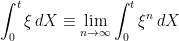
The first thing to do is to define a class of integrable processes for which the integral with respect to ${X}$ is well-defined. Suppose that ${\xi^n}$ is a sequence of predictable processes dominated by any such ${X}$ -integrable process ${\alpha}$ , so that ${\vert\xi^n\vert\le\vert\alpha\vert}$ for each ${n}$ . If this sequence converges to a limit ${\xi}$ , then dominated convergence in probability states that the integrals converge in probability,

$\displaystyle \int_0^t\xi^n\,dX\rightarrow\int_0^t\xi\,dX\ \ \text{(in probability)}$

(1)

as ${n\rightarrow\infty}$ .

We can now define the ${X}$ -integrable processes as the largest class of predictable processes for which dominated convergence can possibly hold. That is, they are `good dominators’. This ensures that we include all possible integrands, and it is easy to show that stochastic integration is indeed well defined for such integrands. The definition necessarily only involves integration with respect to bounded predictable integrands, as that is all we have defined so far.

Definition 1 Let ${X}$ be a semimartingale. Then, ${L^1(X)}$ consists of the set of predictable processes ${\alpha}$ such that, for each ${t\ge 0}$ and sequence of bounded predictable processes ${\xi^n\rightarrow 0}$ with ${\vert\xi^n\vert\le \vert\alpha\vert}$ , then ${\int_0^t\xi^n\,dX\rightarrow 0}$ in probability as ${n\rightarrow \infty}$ .

Alternatively, processes in ${L^1(X)}$ are called ${X}$ -integrable.

Alternative approaches to stochastic integration often define the class of ${X}$ -integrable processes with regard to specific decompositions of ${X}$ . Alternatively, as I shall show in a later post, a predictable process ${\xi}$ is ${X}$ -integrable if and only if

$\displaystyle \left\{\int_0^t\alpha\,dX\colon\vert\alpha\vert\le\vert\xi\vert\text{ is bounded and predictable}\right\}$

is bounded in probability for each ${t\ge 0}$ . However, I prefer the definition above, as it seems to be much more direct and it is clear that all integrands should satisfy this definition. Furthermore, the properties of stochastic integrals follow easily from this. Note that, by bounded convergence, ${L^1(X)}$ includes all bounded predictable processes. As we would hope, it is closed under taking linear combinations.

Lemma 2 Let ${X}$ be a semimartingale. Then, the class of ${X}$ -integrable processes is a vector space. Furthermore, if ${\vert\alpha\vert\le\vert\beta\vert}$ for any predictable process ${\alpha}$ and ${X}$ -integrable process ${\beta}$ , then ${\alpha}$ is also ${X}$ -integrable.

Proof: First, the `furthermore’ statement is a trivial consequence of the definition. To prove the result, it is enough to show that ${\alpha+\beta\in L^1(X)}$ for all ${\alpha,\beta\in L^1(X)}$ . Then, suppose that ${\vert\xi^n\vert\le\vert\alpha+\beta\vert}$ is a sequence of bounded predictable processes tending to zero. Setting

$\displaystyle \alpha^n=\max\left(\min\left(\xi^n,\vert\alpha\vert\right),-\vert\alpha\vert\right),\ \beta^n=\xi^n-\alpha^n$

gives ${\vert\alpha^n\vert\le\vert\alpha\vert}$ and ${\vert\beta^n\vert\le\vert\beta\vert}$ and ${\alpha^n,\beta^n\rightarrow 0}$ . So, applying dominated convergence to ${\alpha^n,\beta^n}$ individually gives

$\displaystyle \int_0^t\xi^n\,dX=\int_0^t\alpha^n\,dX+\int_0^t\beta^n\,dX\rightarrow 0$

in probability as ${n\rightarrow 0}$ . By definition, this shows that ${\alpha+\beta\in L^1(X)}$ . ⬜

Now that we have chosen the largest possible class of predictable processes which can work as integrands, stochastic integration is defined in a similar way as for bounded integrands. That is, it agrees with the explicit expression for the elementary integrands, and satisfies dominated convergence.

Definition 3 Let ${X}$ be a semimartingale and ${t\ge 0}$ . Then, the stochastic integral up to ${t}$ is a map

$\displaystyle L^1(X)\rightarrow L^0,\ \ \xi\mapsto\int_0^t\xi\,dX$

agrees with the explicit expression for elementary integrands.

satisfies dominated convergence in probability (1).

As we would hope, this definition is indeed enough to uniquely specify the stochastic integral.

Lemma 4 Let ${X}$ be a semimartingale. Then, the stochastic integral given by Definition 3 is uniquely defined, is linear in the integrand, and agrees with the previous definition for bounded predictable integrands.

Proof: As ${L^1(X)}$ contains the bounded predictable processes, bounded convergence in probability is just a special case of dominated convergence. So, if it exists, the integral must coincide with that given by the previous definition for bounded integrands.

Conversely, as ${X}$ is a semimartingale, the integral is defined for bounded integrands. It just needs to be extended to all ${X}$ -integrable processes. For any ${\xi\in L^1(X)}$ choose a sequence ${\xi^n\rightarrow\xi}$ of bounded predictable processes which is dominated by some process ${\alpha\in L^1(X)}$ . For example, this can be achieved by setting ${\xi^n=\max(\min(\xi,n),-n)}$ , so ${\vert\xi^n\vert\le\vert\xi\vert}$ . Given such a sequence it follows that ${\xi^m-\xi^n}$ is dominated by ${2\alpha\in L^1(X)}$ and tends to zero as ${m,n\rightarrow\infty}$ . So,

$\displaystyle \int_0^t\xi^m\,dX-\int_0^t\xi^n\,dX = \int_0^t(\xi^m-\xi^n)\,dX\rightarrow 0$

in probability as ${m,n\rightarrow\infty}$ . By completeness under convergence in probability, this allows us to define

$\displaystyle \int_0^t\xi\,dX\equiv\lim_{n\rightarrow\infty}\int_0^t\xi^n\,dX$

(2)

under convergence in probability. It needs to be shown that this definition is independent of the sequence ${\xi^n}$ chosen. So, suppose that ${\zeta^n\rightarrow\xi}$ is any other sequence of bounded predictable processes dominated by some ${\beta\in L^1(X)}$ . Then, ${\xi^n-\zeta^n}$ is dominated by ${\vert\alpha\vert+\vert\beta\vert\in L^1(X)}$ and

$\displaystyle \lim_{n\rightarrow\infty}\int_0^t\xi^n\,dX-\lim_{n\rightarrow\infty}\int_0^t\zeta^n\,dX=\lim_{n\rightarrow\infty}\int_0^t(\xi^n-\zeta^n)\,dX= 0,$

so equation (2) uniquely defines the integral. Furthermore, if ${\xi}$ is bounded, taking ${\xi^n=\xi}$ shows that the integral is consistent with the definition for bounded integrands.

Now, let us prove linearity. If ${\alpha,\beta\in L^1(X)}$ and ${\lambda,\mu}$ are real numbers, then choose sequences of bounded predictable processes ${\alpha^n\rightarrow\alpha}$ , ${\beta^n\rightarrow\beta}$ which are dominated by some ${X}$ -integrable process. As ${L^1(X)}$ is a vector space, ${\lambda\alpha^n+\mu\beta^n}$ will also be dominated by an element of ${L^1(X)}$ . Linearity for bounded integrands gives

$\displaystyle \setlength\arraycolsep{2pt} \begin{array}{rl} \displaystyle\int_0^t(\lambda\alpha+\mu\beta)\,dX &\displaystyle =\lim_{n\rightarrow\infty}\int_0^t(\lambda\alpha^n+\mu\beta^n)\,dX\smallskip\\ &\displaystyle=\lambda\lim_{n\rightarrow\infty}\int_0^t\alpha^n\,dX+\mu\int_0^t\beta^n\,dX\smallskip\\ &\displaystyle =\lambda\int_0^t\alpha\,dX+\mu\int_0^t\beta\,dX \end{array}$

as required.

Finally, we can prove that dominated convergence in probability holds. Let ${\xi^n\rightarrow\xi}$ be predictable processes dominated by some ${\alpha\in L^1(X)}$ . Then, by equation (2), there exist bounded predictable processes ${\vert\alpha^n\vert\le\vert\xi^n-\xi\vert}$ satisfying

$\displaystyle {\mathbb P}\left(\left\vert\int_0^t\alpha^n\,dX-\int_0^t(\xi^n-\xi)\,dX\right\vert>1/n\right)<1/n.$

Then, ${\alpha^n}$ tends to zero and is dominated by ${2\alpha}$ giving,

$\displaystyle \setlength\arraycolsep{2pt} \begin{array}{rl} \displaystyle\int_0^t\xi^n\,dX - \int_0^t\xi\,dX &\displaystyle =\left(\int_0^t(\xi^n-\xi)\,dX-\int_0^t\alpha^n\,dX\right)+\int_0^t\alpha^n\,dX\smallskip\\ &\displaystyle \rightarrow 0 \end{array}$

in probability as ${n\rightarrow\infty}$ , as required. ⬜

Choosing a good version

As stochastic integration of an integrand ${\xi}$ with respect to a semimartingale ${X}$ exists up to all times ${t\ge 0}$ , it defines a new stochastic process ${Y_t\equiv\int_0^t\xi\,dX}$ . Note, however, that the integral takes values in the space ${L^0}$ , of random variables defined up to almost sure equivalence. Therefore, the value of the process ${Y}$ at each time is only defined up to probability one. As discussed in a previous post, this means that the sample paths ${t\mapsto Y_t}$ are not well defined (even up to a set of zero probability), and it is important to choose a good version of the process. In fact, it is always possible to choose cadlag versions of stochastic integrals, which are then uniquely defined up to evanescence. The following result shows that stochastic integrals do indeed have cadlag modifications and, in fact, are semimartingales.

Lemma 5 Let ${X}$ be a semimartingale, ${\xi}$ be an ${X}$ -integrable process, and set ${Y_t=\int_0^t\xi\,dX}$ for each time ${t\ge 0}$ .

Then, ${Y}$ is an adapted process with respect to which the stochastic integral is well defined for all bounded predictable processes, satisfying

$\displaystyle \int_0^t\alpha\,dY=\int_0^t\alpha\xi\,dX.$ (3)

Furthermore, ${Y}$ has a cadlag version.

Proof: For elementary predictable processes ${\xi,\alpha}$ , equality (3) follows directly from the explicit expression for the integrals. It needs to be shown that this extends to all ${X}$ -integrable processes ${\xi}$ , which can be done using the functional monotone class theorem.

Fixing an elementary process ${\alpha}$ , let ${V}$ consist of the set of all ${X}$ -integrable processes ${\xi}$ for which ${Y_t\equiv\int_0^t\xi\,dX}$ is adapted and (3) is satisfied. This includes all elementary predictable processes and, by bounded convergence in probability, is closed under limits of uniformly bounded sequences. Hence, the functional monotone class theorem implies that ${V}$ contains all bounded predictable processes. Then, applying dominated convergence, ${V}$ contains all ${X}$ -integrable processes.

This shows that ${Y}$ is adapted and that equation (3) is satisfied for elementary processes ${\alpha}$ . This needs to be extended to all bounded predictable processes. However, in that case (3) can be used to define the integral with respect to ${Y}$ . Then, dominated convergence applied to integrals with respect to ${X}$ shows that this definition of the integral ${\int_0^t\alpha\,dY}$ does indeed satisfy the bounded convergence theorem, as required. So, by uniqueness of the definition of the stochastic integral, (3) is satisfied.

Finally, as we have shown previously, existence of stochastic integrals with respect to ${Y}$ is enough to imply the existence of a cadlag version. ⬜

Finally, then, the full definition of the stochastic integral is as follows.

Definition 6 Let ${X}$ be a semimartingale. Then, for ${\xi\in L^1(X)}$ , the stochastic integral ${t\mapsto\int_0^t\xi\,dX}$ is a cadlag process satisfying Definition 3 for each fixed time ${t\ge 0}$ .

Notation

I now mention some notation which will be used for the stochastic integral in these notes. When the integral is written without explicitly putting in the limits, then it will refer to the cadlag process rather than the value at any fixed time. E.g., ${Y=\int\xi\,dX}$ is equivalent to ${Y_t=\int_0^t\xi\,dX}$ for each ${t}$ .

Often, the briefer differential notation will be used which, in many situations, can be considerably easier to read. In this notation a differential ${dX}$ just represents a process ${X}$ , up to addition of a constant. Left-multiplication, ${\xi\,dX}$ , represents stochastic integration,

$\displaystyle dY = \xi\,dX\ \Leftrightarrow\ Y=Y_0+\int\xi\,dX.$

10 thoughts on “Extending the Stochastic Integral”

Pingback: The Burkholder-Davis-Gundy Inequality « Almost Sure
Johannes says:

28 February 15 at 12:43 PM

In the proof of Lemma 4 the first definition of \xi^n does not give predictable integrands. What am I missing?

1. Richard Guo says:
  
  26 May 20 at 6:39 AM
  
  $\xi \in L^1(X)$ is predictable by definition, and $\xi^n$ defined as such is predictable.
  
Richard Guo says:

26 May 20 at 6:35 AM

In the proof of Lemma 4, it is not clear to me that the chosen sequence of $\xi^n$ comes with a dominating $\alpha \in L_1(X)$ . Am I missing something?

1. Richard Guo says:
  
  26 May 20 at 6:43 AM
  
  Nevermind… $\xi^n$ is dominated by $\xi$ .
  
Anonymous says:

7 November 23 at 8:13 AM

Could you please elaborate on how you get the bound $|\beta^n|\le |\beta|$ in the proof of Lemma 2?

1. Anonymous says:
  
  19 November 23 at 7:01 PM
  
  It helps to separate the cases β^n > 0 and β^n 0 ⟹ β^n = ξ^n – |α| ≤ |α+β| – |α| ≤ |β| ⟹ |β^n| ≤ |β|.
  
2. Anonymous says:
  
  19 November 23 at 7:03 PM
  
  Ooops.
  
  It helps to separate the cases β^n > 0 and β^n 0, then
  
  β^n = ξ^n – |α| ≤ |α+β| – |α| ≤ |β|,
  
  so |β^n| ≤ |β|. The other case is similar.
  
3. Anonymous says:
  
  19 November 23 at 7:07 PM
  
  That should read:
  
  If β^n > 0, then
  
  β^n = ξ^n – |α| ≤ |α+β| – |α| ≤ |β|
  
  so |β^n| ≤ |β|. The other case is similar.
  
  1. Anonymous says:
    
    23 November 23 at 11:30 PM
    
    Yes, that works. Should also be able to visualise it. Imagine a plot of function ξ^n. α^n is it capped and floored at ±α, and β^n is the amount by which it exceeds the floor/cap. This can’t be more than β, otherwise ξ^n would exceed the |α|+|β| bound

	Anonymous on About
	Anonymous on About
	Anonymous on The Stochastic Integral
	Anonymous on Bessel Processes
	Anonymous on Bessel Processes
	Stat Prof on Pathwise Regularity of Optiona…
	Yang Chu on Spitzer’s Formula
	Anonymous on About
	Anonymous on Continuous Processes with Inde…
	Anonymous on Continuous Processes with Inde…

Extending the Stochastic Integral

Choosing a good version

Notation

Published by George Lowther

10 thoughts on “Extending the Stochastic Integral”

Leave a comment Cancel reply

Choosing a good version

Notation

Related

Published by George Lowther

10 thoughts on “Extending the Stochastic Integral”

Leave a comment Cancel reply