Now that it has been shown that stochastic integration can be performed with respect to any local martingale, we can move on to the following important result. Stochastic integration preserves the local martingale property. At least, this is true under very mild hypotheses. That the martingale property is preserved under integration of bounded elementary processes is straightforward. The generalization to predictable integrands can be achieved using a limiting argument. It is necessary, however, to restrict to locally bounded integrands and, for the sake of generality, I start with local sub and supermartingales.
Theorem 1 Let X be a local submartingale (resp., local supermartingale) and  be a nonnegative and locally bounded predictable process. Then,
  is a local submartingale (resp., local supermartingale).
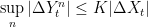
Proof: We only need to consider the case where X is a local submartingale, as the result will also follow for supermartingales by applying to -X. By localization, we may suppose that is uniformly bounded and that X is a proper submartingale. So,  for some constant K. Then, as previously shown there exists a sequence of elementary predictable processes
  such that
  converges to
  in the semimartingale topology and, hence, converges ucp. We may replace
  by
by  if necessary so that, being nonnegative elementary integrals of a submartingale,
  will be submartingales. Also,
  . Recall that a cadlag adapted process X is locally integrable if and only its jump process
  is locally integrable, and all local submartingales are locally integrable. So,
is locally integrable. Then, by ucp convergence for local submartingales, Y will satisfy the local submartingale property. ⬜
For local martingales, applying this result to  gives,
Theorem 2 Let X be a local martingale and be a locally bounded predictable process. Then, is a local martingale.
This result can immediately be extended to the class of local  -integrable martingales, denoted by
  .
.
Corollary 3 Let  for some
  and be a locally bounded predictable process. Then,
 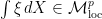 .
.
Continue reading “Preservation of the Local Martingale Property” →

and
be finite measure spaces, and
be a bounded
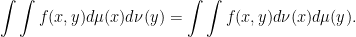
-measurable function. Then,
-measurable,
-measurable, and,

![\displaystyle \setlength\arraycolsep{2pt} \begin{array}{rl} \displaystyle [X]_t&\displaystyle=[X]^c_t+\sum_{s\le t}(\Delta X_s)^2,\smallskip\\ \displaystyle [X,Y]_t&\displaystyle=[X,Y]^c_t+\sum_{s\le t}\Delta X_s\Delta Y_s. \end{array}](https://s0.wp.com/latex.php?latex=%5Cdisplaystyle++%5Csetlength%5Carraycolsep%7B2pt%7D+%5Cbegin%7Barray%7D%7Brl%7D+%5Cdisplaystyle+%5BX%5D_t%26%5Cdisplaystyle%3D%5BX%5D%5Ec_t%2B%5Csum_%7Bs%5Cle+t%7D%28%5CDelta+X_s%29%5E2%2C%5Csmallskip%5C%5C+%5Cdisplaystyle+%5BX%2CY%5D_t%26%5Cdisplaystyle%3D%5BX%2CY%5D%5Ec_t%2B%5Csum_%7Bs%5Cle+t%7D%5CDelta+X_s%5CDelta+Y_s.+%5Cend%7Barray%7D+&bg=ffffff&fg=000000&s=0&c=20201002)
![{[X]^c}](https://s0.wp.com/latex.php?latex=%7B%5BX%5D%5Ec%7D&bg=ffffff&fg=000000&s=0&c=20201002) , is zero. As the only difference between the
, is zero. As the only difference between the ![{[X]^c=0}](https://s0.wp.com/latex.php?latex=%7B%5BX%5D%5Ec%3D0%7D&bg=ffffff&fg=000000&s=0&c=20201002) .
. ![{[X,Y]^c=0}](https://s0.wp.com/latex.php?latex=%7B%5BX%2CY%5D%5Ec%3D0%7D&bg=ffffff&fg=000000&s=0&c=20201002) for all semimartingales Y.
for all semimartingales Y. ![{[X,Y]=0}](https://s0.wp.com/latex.php?latex=%7B%5BX%2CY%5D%3D0%7D&bg=ffffff&fg=000000&s=0&c=20201002) for all continuous semimartingales Y.
for all continuous semimartingales Y. ![{[X,M]=0}](https://s0.wp.com/latex.php?latex=%7B%5BX%2CM%5D%3D0%7D&bg=ffffff&fg=000000&s=0&c=20201002) for all continuous local martingales M.
for all continuous local martingales M.  for a
for a  of FV processes such that
  in the
  is its maximum process.
 there exist positive constants
  such that, for all local martingales X with
  and stopping times
  , the following inequality holds.
 ![\displaystyle c_p{\mathbb E}\left[ [X]^{p/2}_\tau\right]\le{\mathbb E}\left[(X^*_\tau)^p\right]\le C_p{\mathbb E}\left[ [X]^{p/2}_\tau\right].](https://s0.wp.com/latex.php?latex=%5Cdisplaystyle++c_p%7B%5Cmathbb+E%7D%5Cleft%5B+%5BX%5D%5E%7Bp%2F2%7D_%5Ctau%5Cright%5D%5Cle%7B%5Cmathbb+E%7D%5Cleft%5B%28X%5E%2A_%5Ctau%29%5Ep%5Cright%5D%5Cle+C_p%7B%5Cmathbb+E%7D%5Cleft%5B+%5BX%5D%5E%7Bp%2F2%7D_%5Ctau%5Cright%5D.+&bg=ffffff&fg=000000&s=0&c=20201002)
 .
.  , the theorem can also be stated as follows. The set of all cadlag martingales X starting from zero for which
 ![{{\mathbb E}[(X^*_\infty)^p]}](https://s0.wp.com/latex.php?latex=%7B%7B%5Cmathbb+E%7D%5B%28X%5E%2A_%5Cinfty%29%5Ep%5D%7D&bg=ffffff&fg=000000&s=0&c=20201002) is finite is a vector space, and the BDG inequality states that the norms
is finite is a vector space, and the BDG inequality states that the norms ![{X\mapsto\Vert X^*_\infty\Vert_p={\mathbb E}[(X^*_\infty)^p]^{1/p}}](https://s0.wp.com/latex.php?latex=%7BX%5Cmapsto%5CVert+X%5E%2A_%5Cinfty%5CVert_p%3D%7B%5Cmathbb+E%7D%5B%28X%5E%2A_%5Cinfty%29%5Ep%5D%5E%7B1%2Fp%7D%7D&bg=ffffff&fg=000000&s=0&c=20201002) and
and ![{X\mapsto\Vert[X]^{1/2}_\infty\Vert_p}](https://s0.wp.com/latex.php?latex=%7BX%5Cmapsto%5CVert%5BX%5D%5E%7B1%2F2%7D_%5Cinfty%5CVert_p%7D&bg=ffffff&fg=000000&s=0&c=20201002) are equivalent.
are equivalent. ,
,  . The significance of Theorem
  .
.![{\left[\int\xi\,dX\right]=\int\xi^2\,d[X]}](https://s0.wp.com/latex.php?latex=%7B%5Cleft%5B%5Cint%5Cxi%5C%2CdX%5Cright%5D%3D%5Cint%5Cxi%5E2%5C%2Cd%5BX%5D%7D&bg=ffffff&fg=000000&s=0&c=20201002) . Recall, also, that stochastic integration
. Recall, also, that stochastic integration  .
. , so that
 ![{{\mathbb E}[\vert X_t\vert^p]<\infty}](https://s0.wp.com/latex.php?latex=%7B%7B%5Cmathbb+E%7D%5B%5Cvert+X_t%5Cvert%5Ep%5D%3C%5Cinfty%7D&bg=ffffff&fg=000000&s=0&c=20201002) for each t. Then, for any bounded predictable process
for each t. Then, for any bounded predictable process ![\displaystyle \int_0^t\xi^2\,d[X]<\infty](https://s0.wp.com/latex.php?latex=%5Cdisplaystyle++%5Cint_0%5Et%5Cxi%5E2%5C%2Cd%5BX%5D%3C%5Cinfty+&bg=ffffff&fg=000000&s=0&c=20201002)
 .
. ![{[B]_t=t}](https://s0.wp.com/latex.php?latex=%7B%5BB%5D_t%3Dt%7D&bg=ffffff&fg=000000&s=0&c=20201002) and it is easily checked that
and it is easily checked that  is a martingale.
![{X^2-[X]}](https://s0.wp.com/latex.php?latex=%7BX%5E2-%5BX%5D%7D&bg=ffffff&fg=000000&s=0&c=20201002) is a local martingale for all local martingales X.
is a local martingale for all local martingales X. ![\displaystyle XY-[X,Y] = X_0Y_0+\int X_-\,dY+\int Y_-\,dX](https://s0.wp.com/latex.php?latex=%5Cdisplaystyle++XY-%5BX%2CY%5D+%3D+X_0Y_0%2B%5Cint+X_-%5C%2CdY%2B%5Cint+Y_-%5C%2CdX+&bg=ffffff&fg=000000&s=0&c=20201002)
 , is said to converge to a process X under the
  should tend to
  in probability. Also, for every sequence
  of
of  ,
,
 .
. for some
  if and only if there is a sequence
  .
.  for its closure under the semimartingale topology, the statement of the theorem is equivalent to
 were defined to be
  and
and  pointwise, then
  tends to zero in probability. This definition is a bit messy. Fortunately, the following result gives a much cleaner characterization of X-integrability.
 .
.  ,
,  denotes the bounded
  -measurable functions
  . For a
  satisfying the following bounded convergence property; if a sequence
  (n=1,2,…) is uniformly bounded, so that
  for a constant K, and converges pointwise to a limit
  , then
  in V.
in V. satisfying
  satisfying bounded convergence and, conversely, any linear map
  . So, these definitions are essentially the same, but for the purposes of these notes it is more useful to represent V-valued measures in terms of their integrals rather than the values on measurable sets.
 be a subalgebra of
  extends to a V-valued measure on
  .
.  then
then  .
. , then