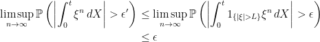
Further Properties of the Stochastic Integral

We move on to properties of stochastic integration which, while being fairly elementary, are rather difficult to prove directly from the definitions.

First, recall that for a semimartingale X, the X-integrable processes ${L^1(X)}$ were defined to be predictable processes ${\xi}$ which are ‘good dominators’. That is, if ${\xi^n}$ are bounded predictable processes with ${\vert\xi^n\vert\le\vert\xi\vert}$ and ${\xi^n\rightarrow 0}$ pointwise, then ${\int_0^t\xi^n\,dX}$ tends to zero in probability. This definition is a bit messy. Fortunately, the following result gives a much cleaner characterization of X-integrability.

Theorem 1 Let X be a semimartingale. Then, a predictable process ${\xi}$ is X-integrable if and only if the set

$\displaystyle \left\{\int_0^t\zeta\,dX\colon\zeta\in{\rm b}\mathcal{P},\vert\zeta\vert\le\vert\xi\vert\right\}$ (1)

is bounded in probability for each ${t\ge 0}$ .

Proof: That it is necessary for the set in (1) to be bounded in probability follows from dominated convergence. If ${\zeta^n\in{\rm b}\mathcal{P}}$ satisfy ${\vert\zeta^n\vert\le\vert\xi\vert}$ and ${\lambda_n\in{\mathbb R}}$ go to zero, then ${\lambda_n\zeta^n\rightarrow 0}$ and dominated convergence gives ${\lambda_n\int_0^t\zeta^n\,dX\rightarrow 0}$ in probability. By the sequential characterization of boundedness, the given set is indeed bounded in probability.

Conversely, suppose that the set in (1) is bounded in probability. It needs to be shown that, for any sequence ${\xi^n\in{\rm b}\mathcal{P}}$ with ${\vert\xi^n\vert\le\vert\xi\vert}$ and ${\xi^n\rightarrow 0}$ then ${\int_0^t\xi^n\,dX\rightarrow 0}$ in probability.

First, suppose that ${\sum_n\vert\xi^n\vert\le\vert\xi\vert}$ . Choosing any ${\epsilon_1,\ldots,\epsilon_n\in\{1,-1\}}$ then ${\sum_{k=1}^n\epsilon_k\xi^k}$ is bounded by ${\xi}$ . So, the collection of all sums of the form

$\displaystyle \sum_{k=1}^n\epsilon_k\int_0^t\xi^k\,dX$

is in the set (1) and, hence, is bounded in probability. Using Lemma 4 in the construction of the stochastic integral, this is enough to conclude that ${\int_0^t\xi^k\,dX}$ tends to zero in probability.

Choosing any ${\epsilon>0}$ we can now show, by contradiction, that there is a positive constant L with ${{\mathbb P}(\vert\int_0^t 1_{\{\vert\xi\vert>L\}}\zeta\,dX\vert>\epsilon)\le\epsilon}$ for all bounded predictable processes ${\vert\zeta\vert\le\vert\xi\vert}$ . If this was not the case, then for any increasing sequence of numbers ${L_n\uparrow\infty}$ there would exist bounded predictable ${\vert\zeta^n\vert\le\vert\xi\vert}$ such that

$\displaystyle {\mathbb P}\left(\left\vert\int_0^t1_{\{\vert\xi\vert>L_n\}}\zeta^n\,dX\right\vert>\epsilon\right)>\epsilon.$

(2)

Furthermore, by bounded convergence, (2) still holds if ${\zeta^n}$ is replaced by ${1_{\{\vert\xi\vert\le L_m\}}\zeta^n}$ for large enough m. Then, by passing to a subsequence if necessary, we may suppose that ${1_{\{\vert\xi\vert>L_{n+1}\}}\zeta^n=0}$ . So,

$\displaystyle \sum_{n=1}^\infty 1_{\{\vert\xi\vert>L_n\}}\vert\zeta^n\vert\le\sum_{n=1}^\infty 1_{\{L_{n+1}\ge\vert\xi\vert>L_n\}}\vert\xi\vert\le\vert\xi\vert$

so that, by the above argument, ${\int_0^t1_{\{\vert\xi\vert>L_n\}}\zeta^n\,dX}$ tends to zero in probability, contradicting (2).

Now, suppose that L is as above and that ${\vert\xi^n\vert\le\vert\xi\vert}$ tend to zero. By bounded convergence, ${\int_0^t1_{\{\vert\xi\vert\le L\}}\xi^n\,dX}$ tends to zero in probability and,

$\displaystyle \setlength\arraycolsep{2pt} \begin{array}{rl} \displaystyle\limsup_{n\rightarrow\infty}{\mathbb P}\left(\left\vert\int_0^t\xi^n\,dX\right\vert>\epsilon^\prime\right)&\displaystyle\le\limsup_{n\rightarrow\infty}{\mathbb P}\left(\left\vert\int_0^t 1_{\{\vert\xi\vert>L\}}\xi^n\,dX\right\vert>\epsilon\right)\smallskip\\ &\displaystyle\le\epsilon \end{array}$

for all ${\epsilon^\prime>\epsilon}$ . As ${\epsilon>0}$ was arbitrary, this shows that ${\int_0^t\xi^n\,dX\rightarrow 0}$ in probability as required. ⬜

Changes of Filtration

Recall that we work with respect to a complete filtered probability space ${(\Omega,\mathcal{F},\{\mathcal{F}_t\}_{t\ge 0},{\mathbb P})}$ . Sometimes it can be useful to replace ${F\equiv\{\mathcal{F}_t\}_{t\ge 0}}$ by an alternative filtration ${G=\{\mathcal{G}_t\}_{t\ge 0}}$ , while keeping the same underlying probability space ${(\Omega,\mathcal{F},{\mathbb P})}$ . It is assumed that ${\mathcal{G}_t\subseteq\mathcal{F}}$ , so changing filtrations in this way gives a new filtered probability space ${(\Omega,\mathcal{F},G,{\mathbb P})}$ . For example, if studying a process which is not adapted, changing to a new filtration with respect to which it is adapted can be useful technique.

Changing filtrations in this way affects the notion of adapted processes and, therefore, the space of predictable processes changes. As stochastic integration was defined only for predictable integrands, it is also affected by changes of filtration. If a process X is a semimartingale with respect to F, it can fail to be a semimartingale with respect to a different filtration G even in the case where X is also G-adapted. Even if it is, the space of X-integrable processes and the values of the stochastic integral can differ.

I will say F-predictable, F-semimartingale, etc to denote that the respective property holds with respect to a given filtration F. Also, if X is an F-semimartingale, ${L^1(X,F)}$ denotes the X-integrable processes with respect to F.

The filtration G is said to be a subfiltration of F if ${\mathcal{G}_t\subseteq\mathcal{F}_t}$ for each t. This case is particularly easy, because passing to a subfiltration reduces the set of predictable processes, making it easier for there to be a well defined stochastic integral.

Theorem 2 (Stricker’s Theorem) Let X be a semimartingale for the filtration F, and G be a subfiltration of F such that X is G-adapted. Then, X is a G-semimartingale.

Furthermore, if ${\xi\in L^1(X,F)\cap L^1(X,G)}$ then the integrals ${\int\xi\,dX}$ defined with respect to F and G agree.

Proof: As G is a subfiltration of F, every G-predictable process is also F-predictable. We can therefore define the integral ${\int\xi\,dX}$ for bounded G-predictable ${\xi}$ to be equivalent to the value defined with respect to F. This agrees with the explicit expression for G-elementary processes and satisfies bounded convergence in probability.

So, X is a G-semimartingale by definition and the stochastic integral defined under G for bounded integrands agrees with the definition under F. Now, suppose that ${\xi\in L^1(X,F)\cap L^1(X,G)}$ . Then, dominated convergence

$\displaystyle \int\xi\,dX=\lim_{n\rightarrow\infty}\int(\xi\wedge n)\vee(-n)\,dX$

applies under both filtrations, and the two definitions of the integral agree. ⬜

Going in the opposite direction and increasing the size of the filtration makes the set of predictable processes larger, so it becomes less likely that there is a well-defined stochastic integral. For example, a standard Brownian motion is a semimartingale under its natural filtration but, as it has infinite variation on bounded sets, it is not a semimartingale under the maximal filtration (where ${\mathcal{G}_t=\mathcal{F}}$ for all t).

However, enlarging the filtration by adding a single set to ${\mathcal{F}_t}$ , the semimartingale property is preserved. In fact, enlarging the filtration by any countable collection of disjoint sets preserves the semimartingale property. This is known as Jacod’s Countable Expansion. Furthermore, X-integrability is also preserved.

Theorem 3 Let ${A_1,A_2,\ldots}$ be a sequence of pairwise disjoint sets in ${\mathcal{F}}$ and, for each t, let ${\mathcal{G}_t}$ be the sigma algebra generated by ${\mathcal{F}_t\cup\{A_n\colon n=1,2,\ldots\}}$ . So, ${{\rm G}=\{\mathcal{G}_t\}_{t\ge 0}}$ is a filtration containing F.

Then, every F-semimartingale X is also a G-semimartingale. Furthermore, ${L^1(X,F)\subseteq L^1(X,G)}$ and, for ${\xi\in L^1(X,F)}$ , the definitions of the integral ${\int\xi\,dX}$ with respect to F and G agree.

Proof: First, by inserting ${\Omega\setminus\bigcup_nA_n}$ into the sequence of sets, we can suppose that ${\bigcup_nA_n=\Omega}$ . I make use of the result that a set S of random variables is bounded in probability if and only if ${1_{A_n}S\equiv\{1_{A_n}U\colon U\in S\}}$ is bounded in probability for each n.

The enlarged filtration G and its associated predictable processes are not hard to describe. First, ${\mathcal{G}_t}$ is the collection of sets of the form ${\bigcup_n(A_n\cap B_n)}$ for ${B_n\in\mathcal{F}_t}$ . The ${\mathcal{G}_t}$ -measurable random variables are of the form ${\sum_n1_{A_n}Z_n}$ for ${\mathcal{F}_t}$ -measurable random variables ${Z_n}$ . Then, the G-elementary processes are ${\sum_n1_{A_n}\xi^n}$ for F-elementary processes ${\xi^n}$ . Similarly, the G-predictable processes are of the form ${\sum_n1_{A_n}\xi^n}$ for F-predictable ${\xi^n}$ .

The characterization of semimartingales in terms of boundedness in probability will be used. Suppose that X is an F-semimartingale and, for each t, define the sets

$\displaystyle \setlength\arraycolsep{2pt} \begin{array}{rl} &\displaystyle S = \left\{\int_0^t\xi\,dX\colon\vert\xi\vert\le 1,\xi\text{\ is\ F-elementary}\right\}\smallskip\\ &\displaystyle S' = \left\{\int_0^t\xi\,dX\colon\vert\xi\vert\le 1,\xi\text{\ is\ G-elementary}\right\} \end{array}$

For any G-elementary process ${\vert\xi\vert\le 1}$ , there are F-elementary processes ${\xi^n}$ with ${1_{A_n}\xi=1_{A_n}\xi^n}$ . Replacing ${\xi^n}$ by ${(\xi^n\wedge 1)\vee(-1)}$ , we suppose that ${\vert\xi^n\vert\le 1}$ . Then, ${1_{A_n}\int_0^t\xi\,dX=1_{A_n}\int_0^t\xi^n\,dX}$ . So, ${1_{A_n}S^\prime\subseteq 1_{A_n}S}$ .

The following implications hold. X is an F-semimartingale implies that S is bounded in probability, implying that ${1_{A_n}S}$ are bounded in probability, so ${1_{A_n}S^\prime}$ are bounded in probability. Then, ${S^\prime}$ is bounded in probability and X is a G-semimartingale.

It only remains to prove that ${L^1(X,F)\subseteq L^1(X,G)}$ , in which case the agreement of stochastic integration defined with respect to F and G comes from Theorem 2.

The proof that X-integrability is preserved when enlarging the filtration follows in a similar way as for the semimartingale property above. The characterization of X-integrability in terms of boundedness in probability given by Theorem 1 is used. So, suppose that ${\xi\in L^1(X,F)}$ and define

$\displaystyle \setlength\arraycolsep{2pt} \begin{array}{rl} &\displaystyle S = \left\{\int_0^t\zeta\,dX\colon\vert\zeta\vert\le\vert\xi\vert,\zeta\text{\ is bounded, F-predictable},\right\}\smallskip\\ &\displaystyle S' = \left\{\int_0^t\zeta\,dX\colon\vert\zeta\vert\le\vert\xi\vert,\zeta\text{\ is bounded, G-predictable}\right\}. \end{array}$

For any bounded G-predictable process ${\vert\zeta\vert\le\vert\xi\vert}$ , there are bounded F-predictable ${\zeta^n}$ such that ${1_{A_n}\zeta=1_{A_n}\zeta^n}$ . Replacing ${\zeta^n}$ by ${(\zeta^n\wedge\vert\xi\vert)\vee(-\vert\xi\vert)}$ , we suppose that ${\vert\zeta^n\vert\le\vert\xi\vert}$ . Then, ${1_{A_n}\int_0^t\zeta\,dX=1_{A_n}\int_0^t\zeta^n\,dX}$ , proving that ${1_{A_n}S^\prime\subseteq 1_{A_n}S}$ .

In a similar way to the proof above, ${S}$ is bounded in probability implies ${1_{A_n}S}$ are bounded in probability, implying that ${1_{A_n}S^\prime}$ are bounded in probability, so ${S^\prime}$ is bounded in probability and ${\xi\in L^1(X,G)}$ . ⬜

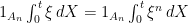
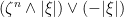
Finally, for this post, we prove the following ‘pathwise’ property of stochastic integration. The stochastic integrals with respect to two different integrands agree on any measurable set for which the integrands agree. If integration was defined in a pathwise manner, such as when taking the standard Stieltjes integrals with respect to finite variation processes, then this result would be immediate. However, it appears to be very difficult to prove from the defining properties of stochastic integration. Instead, Theorem 3 above is used which, in turn, relied on the alternative definition of semimartingales in terms of boundedness in probability.

Theorem 4 Let X be a semimartingale and ${\xi,\zeta\in L^1(X)}$ . If ${A\in\mathcal{F}}$ is any set such that ${\xi=\zeta}$ on A, then ${\int\xi\,dX=\int\zeta\,dX}$ on A.

Proof: Using Theorem 3, enlarge the filtration by adding the set A to each ${\mathcal{F}_t}$ . Working with respect to this larger filtration, ${1_A\xi=1_A\zeta}$ are X-integrable and,

$\displaystyle 1_A\int\xi\,dX=\int 1_A\xi\,dX = \int 1_A\zeta\,dX = 1_A\int\zeta\,dX$

as required. ⬜

Notes

The characterization of X-integrable processes given by Theorem 1 is a bit different those used in most introductions to stochastic calculus. The usual approach is to decompose the semimartingale X=M+V into a local martingale part M and FV term V. Then, a process is X-integrable if it is both V-integrable in the Lebesgue-Stieltjes sense and M-integrable according to the construction of stochastic integrals with respect to local martingales. However, such decompositions are not unique, and different decompositions lead to different sets of integrands. Then, a process is said to be X-integrable if it is integrable with respect to at least one such decomposition. It can be shown that this does give the same class of integrands as in Theorem 1, but it is not easy to prove this.

On the other hand, Theorem 1 gives what seems to be a more natural and intrinsic definition of X-integrability. I’m not sure if the result that this is a necessary and sufficient condition is new, and am not aware of any authors using this characterization. It does seem surprising if this is the case, as it is such a simple definition of X-integrable processes.

5 thoughts on “Further Properties of the Stochastic Integral”

TheBridge says:

25 October 11 at 1:28 PM

Hi,

About the fact that you mention that a Brownian motion is not a semimartingale under the maximal filtration. You argue that it is because it has infinite variations over bounded sets.

As I understand it, if we use the Bichteler-Dellacherie Decomposition Theorem of semimartingales, and as a Brownian Motion under this filtration has no local martingale part (because it is an a.s. non constant deterministic process in this filtration), if it were a semimartingale then it should be a FV process which is false by properties of Brownian Motion paths, so making the desired contradiction appear.

The thing is that Bichteler-Dellacherie Decomposition Theorem only appears much later in these notes so I was wondering if there was a simpler argument.

Best regards

1. George Lowther says:
  
  25 October 11 at 6:50 PM
  
  Ok, I stated it here as fact, but you can easily show that if X is any process and the filtration is large enough that X_t is $\mathcal{F}_0$ -measurable for all t ≥ 0, then X is a semimartingale if and only if it is cadlag with finite variation on each bounded interval.
  
  If 0 = t₀ ≤ t₁ ≤ ⋯ ≤ t_n = T is a partition of the interval [0,T] then
  
  $\displaystyle\xi_t=\sum_{k=1}^n1_{\{t_{k-1} < t\le t_k\}}{\rm sgn}(X_{t_k}-X_{t_{k-1}})$
  
  is a predictable process bounded by 1. The integral is
  
  $\displaystyle\int_0^T\xi\,dX=\sum_{k=1}^n\vert X_{t_k}-X_{t_{k-1}}\vert.$
  
  If X was a semimartingale then this would be bounded (in probability) independently of the choice of partition. However, as the mesh max|t_k – t_k-1| goes to zero, it tends to the variation of X on the interval [0,T]. So, if X is a semimartingale then its sample paths almost surely have finite variation on each interval [0,T].
  
  1. TheBridge says:
    
    25 October 11 at 7:57 PM
    
    Ok thanks this very elegant argument.
    Best Regards
    
Ilya Zakharevich says:

22 March 21 at 3:23 AM

Misprints:
(A) look for misparsed backticks (search for ticks, as in `good dominators’).
(B) look for
and.
with a trailing dot.

(It seems that (A) is a property of a font. At least on Windows it is shown fine in FF or Chrome, but on Android v4 it is shown as a diacritical mark. Still, using proper backquote — as opposed to ASCII backticks — would be better.)

1. George Lowther says:
  
  24 March 21 at 9:32 AM
  
  Ok, thanks, updated these. WordPress seems to do some processing of quote marks. I’m not sure if the way it does this has changed, but the issue with backticks is in all of my older posts, and I will update when I have time.

	Tavin on Class (D) Processes
	George Lowther on Filtrations and Adapted P…
	faceet on Filtrations and Adapted P…
	George Lowther on Filtrations and Adapted P…
	facet on Filtrations and Adapted P…
	Zoltan on Class (D) Processes
	Zoltan on Class (D) Processes
	ARS on Stopping Times and the Debut…
	George Lowther on Upcrossings, Downcrossings, an…
	George Lowther on Stopping Times and the Debut…

Further Properties of the Stochastic Integral

Changes of Filtration

Notes

Published by George Lowther

5 thoughts on “Further Properties of the Stochastic Integral”

Leave a Reply Cancel reply

Changes of Filtration

Notes

Like this:

Related

Published by George Lowther

5 thoughts on “Further Properties of the Stochastic Integral”

Leave a Reply Cancel reply