The construction of the stochastic integral given in the previous post made use of a result showing that certain linear maps can be extended to vector valued measures. This result, Theorem 1 below, was separated out from the main argument in the construction of the integral, as it only involves pure measure theory and no stochastic calculus. For completeness of these notes, I provide a proof of this now.
Given a measurable space  ,
,  denotes the bounded
  -measurable functions
  . For a topological vector space V, the term V-valued measure refers to linear maps
  satisfying the following bounded convergence property; if a sequence
  (n=1,2,…) is uniformly bounded, so that
  for a constant K, and converges pointwise to a limit
  , then
  in V.
in V.
This differs slightly from the definition of V-valued measures as set functions  satisfying countable additivity. However, any such set function also defines an integral
  satisfying bounded convergence and, conversely, any linear map satisfying bounded convergence defines a countably additive set function
  . So, these definitions are essentially the same, but for the purposes of these notes it is more useful to represent V-valued measures in terms of their integrals rather than the values on measurable sets.
In the following, a subalgebra of is a subset closed under linear combinations and pointwise multiplication, and containing the constant functions.
Theorem 1 Let be a measurable space,  be a subalgebra of generating , and V be a complete vector space. Then, a linear map
  extends to a V-valued measure on if and only if it satisfies the following properties for sequences
  .
.
- If
 then
then  .
.
- If
 , then .
The conditions stated are necessary for the existence of an extension to a V-valued measure because, in both cases,  is a uniformly bounded sequence converging to 0. Note the similarity of this result to Carathéodory’s extension theorem for standard (real-valued) measures. Suppose that are linear combinations of indicator functions 1A for A in some subset
  which is closed under finite intersections and under complements. Then, setting
  , the conditions of the theorem are equivalent to the requirement that
  whenever
  are either pairwise disjoint or decreasing to the empty set.
The construction of the stochastic integral only made use of the special case where  is the predictable sigma algebra,
  is the space of random variables (up to almost sure equivalence) under convergence in probability, and is the set of uniformly bounded continuous and adapted processes. However, it is not much more difficult to prove Theorem 1 in full generality, which we do here.
First, if satisfy  then so that, by the second condition of the theorem, . It follows that
  is continuous under the topology of uniform convergence on and, by continuous linear extensions, extends uniquely to a continuous linear function from the closure
  of under uniform convergence. As is an algebra,
  for every polynomial p and
  . The Stone-Weierstrass theorem states that continuous functions on a bounded interval can be uniformly approximated by polynomials, so
  for all continuous functions
  and . Furthermore, this extension of still satisfies the conditions of the theorem. If
  , then choose
  with
with  . If then
  will also be decreasing to zero, giving
  . Alternatively, if then
  , again giving . In either case,
  tends to zero as required. So, by passing to the closure if necessary, it may be assumed that is closed under uniform convergence.
Throughout the remainder of this post, it is assumed that is closed under uniform convergence. So,  for continuous functions and
  . In particular, we make use of the fact that the absolute value
  of any is itself in .
The proof I give here is close to the construction of the stochastic integral given by Bichteler in Stochastic Integration and Lp-Theory of Semimartingales and in his book, `Stochastic Integration with Jumps’. The idea is to define a semimetric D* on the bounded measurable functions, referred to by Bichteler as the Daniell mean. Once it is shown that is continuous under this metric, a continuous linear extension to the whole of can be used. Let us suppose that the topology on V is given by a translation invariant metric  . This is indeed true in the construction of the stochastic integral, where and
 ![{D(U)\equiv{\mathbb E}[\vert U\vert\wedge 1]}](https://s0.wp.com/latex.php?latex=%7BD%28U%29%5Cequiv%7B%5Cmathbb+E%7D%5B%5Cvert+U%5Cvert%5Cwedge+1%5D%7D&bg=ffffff&fg=000000&s=0&c=20201002) generates the topology of convergence in probability. Generalizing to arbitrary complete vector spaces is straightforward, as demonstrated in the subsection below. By the standard metric properties, D must satisfy
generates the topology of convergence in probability. Generalizing to arbitrary complete vector spaces is straightforward, as demonstrated in the subsection below. By the standard metric properties, D must satisfy  and
and  for all u,v in V. Furthermore, replacing D(v) by min(D(v),1) if required, we suppose that D is bounded.
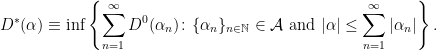
For any , define
Then, define  by
by
 |
(1) |
Although I have used a slightly different definition, this is the quantity referred to as the Daniell mean by Bichteler. In fact, D* and D0 will agree on , as we show in a moment. Countable subadditivity follows from this definition in a straightforward way, as given by the following lemma. In particular, the triangle inequality  is satisfied, so D* defines a translation invariant semimetric on .
Lemma 2 Suppose that  satisfy
  . Then,
 |
(2) |
Proof: Using (1), for any  there exist
  satisfying
  and
and
As  ,
,
As was arbitrary, (2) follows. ⬜
Let us also show that D* and D0 agree on . In particular, this gives  , so that is continuous with respect to the semimetric D*.
Lemma 3 For any ,
Proof: Setting  and
and  for n=2,3,… in (1) gives
  , so only the reverse inequality needs to be shown.
Given any  with
with  , setting
  and
and  gives
gives  and
and  . So,
. So,
Taking the supremum over all gives the triangle inequality,
Now choose a sequence with and set  . For any
  with
with  , set
, set  so that
  .
.
Then,  and
and  decrease monotonically to zero. So, by the first property of Theorem 1,
Then, applying the triangle inequality for D0, we obtain the following
Taking the infimum over all such and applying (1) gives  . Then taking the supremum over gives
  as required. ⬜
Now, let  be the closure of with respect to the topology generated by the semimetric D*. That is,
  if and only if there is a sequence such that
  . Then, D* satisfies monotone convergence on
  .
.
Lemma 4 Let  and
and  be such that
  . Then, and .
Proof: First, let us show that  as m,n go to infinity. Choose any and with
  . Suppose that
  for some constant K. Replacing
  by
by  if necessary, we may suppose that
  . Then, setting
  ,
,
So,  is bounded below by
  and above by
  . Applying the triangle inequality,
Summing over n=2,…,m gives
Now, choose any sequence  . As
. As  is increasing,
  has a sum bounded by K. So, any
  with
with  also have a sum bounded by K and, by the second condition of Theorem 1,
  . By Lemma 3, we can choose
  , showing that
  . Since the sequence was arbitrary, this shows that
  as m,n go to infinity. So,
As was arbitrary, this shows that  as required.
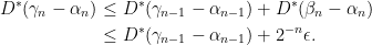
Now choosing such that  whenever
  then, for
  , countable subadditivity (Lemma 2) gives
which goes to 0 as k increases to infinity. ⬜
Putting together the previous lemmas, it is now straightforward to show that is the whole of and that D* satisfies bounded convergence.
Lemma 5 The equality  holds. Furthermore, suppose that are uniformly bounded by some constant K, so that , and
  pointwise as n goes to infinity. Then, .
Proof: As is a linear space closed under monotone limits (by Lemma 4), and contains the algebra generating , the monotone class theorem says that .
Now, suppose that satisfy and  . The sequence
  decreases monotonically to zero. So,
  and Lemma 4 gives
  . Therefore,
as required. ⬜
The extension of to a V-valued measure is finally given by a continuous linear extension, completing the proof of Theorem 1.
Lemma 6 Let V be a complete vector space, with translation invariant metric D. Then, assuming the conditions of Theorem 1, extends uniquely to a V-valued measure on .
Proof: Define the semimetric D* on as in (1). By Lemma 3, . So, is D*/D-continuous and extends uniquely to a continuous linear function  which, by Lemma 5, satisfies the bounded convergence property. ⬜
Generalizing to arbitrary complete vector spaces
The proof of Theorem 1 can be extended to arbitrary complete vector spaces, not given by a translation invariant metric. This is not needed for the construction of the stochastic integral, but it is not difficult, and I do this now for the sake of giving a full proof of the theorem as stated. We can use the result that any vector topology is given by a collection of translation invariant semimetrics  . As above, replacing Di(v) by min(Di(v),1), we may suppose that Di are bounded. Then, by the above argument, there is a collection
  of semimetrics on such that
  for all , and satisfying bounded convergence as in Lemma 5.
Then, the closure of with respect to the topology generated by is a linear space closed under monotone convergence (by Lemma 4) and, by the monotone class theorem, is the whole of . By continuous linear extensions, extends uniquely to a continuous linear function . By Lemma 5,  satisfies bounded convergence and hence is a V-valued measure.
The statement that all vector topologies are generated by a set of translation invariant semimetrics needs some explanation. It is a standard result of functional analysis that a vector topology is given by such a semimetric if and only if it has a countable base of neighborhoods of the origin. Then, for an aribitrary vector topology  , let
, let  be a base of balanced neighborhoods of the origin. For each i, by the properties of vector topologies, there is a sequence of balanced neighborhoods of the origin Ui,n such that
  and Ui,n=Ui. Again, by standard results of functional analysis,
  generate a vector topology which will then be generated by some translation invariant semimetric Di. The set generates as required.


Hi
Two questions, on this very interesting topic: in Theorem 1 ?
– What do you mean exactly by “generating
– Where can I find a book where this theorem is stated ? This is the first time I see integration presented this way.
Regards
Hi. generates
  I mean that
  is the smallest σ-algebra with respect to which every
  is measurable. By the monotone class theorem, this is equivalent to
  being the smallest collection of functions
  containing
  and closed under taking limits of uniformly bounded monotone sequences.
By saying that
I don’t have a precise reference for Theorem 1.
The treatment of stochastic integration in this and the previous post is based very roughly on that given by Bichteler in the book Stochastic Integration with Jumps, and he has a freely downloadable version on his website. However, the way in which I arrange the proof here is largely my own, so Theorem 1 is not quoted from any other source. The main trick which I used here from Bichteler’s method is the use of the Khintchine inequality (Lemma 3 of the previous post). This guarantees that the stochastic integral satisfies the second statement of Theorem 1 above. My proof of existence of the stochastic integral is organized rather differently from Bichteler’s though. I split out the part of the construction which depends on the specific properties of the stochastic integral (in the previous post) from the part which works for arbitrary vector valued measures (Theorem 1 above).
You could take a look at The Carathéodory extension theorem for vector valued measures. The main theorem quoted there is very similar to Theorem 1, except that it is stated for Banach spaces (so not L0) and is for actual vector measures, rather than the σ-additive linear functions here.
Just as the Riemann–Stieltjes integral can be equivalently defined as a Lebesgue integral with the corresponding Lebesgue–Stieltjes measure, I am looking for similar/corresponding results for the relationship between Stochastic integrals (both Ito and Stratonovich) and Bochner Integrals (or any other integral taking values in Banach spaces). I’m also looking for results on the corresponding measure defined on the relevant Banach Spaces.
Information pertaining to Stochastic integrals with integration with respect to Brownian motion is more than welcome, but I am looking for results pertaining more to integrals with integration in respect to more general semi-martingales. Any references or results you can forward to me is greatly appreciated. Thanks.