
The principal reason for introducing the concept of semimartingales in stochastic calculus is that they are precisely those processes with respect to which stochastic integration is well defined. Often, semimartingales are defined in terms of decompositions into martingale and finite variation components. Here, I have taken a different approach, and simply defined semimartingales to be processes with respect to which a stochastic integral exists satisfying some necessary properties. That is, integration must agree with the explicit form for piecewise constant elementary integrands, and must satisfy a bounded convergence condition. If it exists, then such an integral is uniquely defined. Furthermore, whatever method is used to actually construct the integral is unimportant to many applications. Only its elementary properties are required to develop a theory of stochastic calculus, as demonstrated in the previous posts on integration by parts, Ito’s lemma and stochastic differential equations.
The purpose of this post is to give an alternative characterization of semimartingales in terms of a simple and seemingly rather weak condition, stated in Theorem 1 below. The necessity of this condition follows from the requirement of integration to satisfy a bounded convergence property, as was commented on in the original post on stochastic integration. That it is also a sufficient condition is the main focus of this post. The aim is to show that the existence of the stochastic integral follows in a relatively direct way, requiring mainly just standard measure theory and no deep results on stochastic processes.
Recall that throughout these notes, we work with respect to a complete filtered probability space 
 |
(1) |
for an 


 |
(2) |
The predictable sigma algebra, 


Using the definition of a semimartingale as a cadlag adapted process with respect to which the stochastic integral is well defined for bounded and predictable integrands, the main result is as follows. To be clear, in this post all stochastic processes are real-valued.
Theorem 1 A cadlag adapted process X is a semimartingale if and only if, for each
, the set
(3)
is bounded in probability.

As was previously noted, the necessity of this condition follows from bounded convergence. In fact, boundedness in probability of the set in (3) is equivalent to the statement that, for any sequence 

The proof of Theorem 1 is given below. However, it helps to take a step back at this point and ask the following question. What do we need to do, in general, to construct linear maps satisfying bounded convergence of sequences? This question is not restricted to stochastic calculus, and can be asked in a much more general situation. Given a measurable space 


Theorem 2 Let
be a subalgebra of
, and V be a complete vector space. Then, a linear map
extends to a V-valued measure on
.
- If
then
.
- If
, then
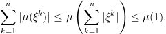
The proof of this result will be given in the next post, as the details would cloud the main argument here and, in any case, it is just a statement involving pure measure theory with no stochastic calculus whatsoever. Both of the conditions of this theorem involve a uniformly bounded sequence 
It is instructive to pause here for a moment, and consider how these conditions are shown to be true in the case of Lebesgue integration and Stieltjes integration with respect to finite variation functions, and to compare with the stochastic case. The first condition, of monotone convergence, can be shown by making use of the compactness of the interval ![{[0,t]}](https://s0.wp.com/latex.php?latex=%7B%5B0%2Ct%5D%7D&bg=ffffff&fg=000000&s=0&c=20201002)
The second condition of Theorem 2 is really where the difference between standard integration and the stochastic integral comes in. Consider, for example, the usual Lebesgue integral on the interval 

 |
It follows that 
Similarly, if 


 |
(4) |
So, once again, 
This argument does not apply to stochastic integration, which takes values in the space 


However, it turns out that a modified argument along similar lines does indeed work for stochastic integration and, more generally, for all vector-valued measures taking values in a space 


Suppose that 


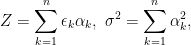 |
(5) |
so that Z has mean zero and variance 
Lemma 3 Given a real number
, there exists a
such that for any
of the form (5),
Here,
only depends on K and not on the choice of

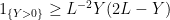
Proof: We shall make use of the inequality
![\displaystyle {\mathbb P}(Y> 0)\ge{\mathbb E}[Y]^2/{\mathbb E}[Y^2].](https://s0.wp.com/latex.php?latex=%5Cdisplaystyle++%7B%5Cmathbb+P%7D%28Y%3E+0%29%5Cge%7B%5Cmathbb+E%7D%5BY%5D%5E2%2F%7B%5Cmathbb+E%7D%5BY%5E2%5D.+&bg=ffffff&fg=000000&s=0&c=20201002) |
(6) |
This holds for any integrable random variable 
![{{\mathbb E}[Y^2]/{\mathbb E}[Y]}](https://s0.wp.com/latex.php?latex=%7B%7B%5Cmathbb+E%7D%5BY%5E2%5D%2F%7B%5Cmathbb+E%7D%5BY%5D%7D&bg=ffffff&fg=000000&s=0&c=20201002)

Now use the properties that 
![{{\mathbb E}[Z^2]=\sigma^2}](https://s0.wp.com/latex.php?latex=%7B%7B%5Cmathbb+E%7D%5BZ%5E2%5D%3D%5Csigma%5E2%7D&bg=ffffff&fg=000000&s=0&c=20201002)
![\displaystyle \setlength\arraycolsep{2pt} \begin{array}{rl} \displaystyle{\mathbb E}[Z^4] &\displaystyle=3\sum_{j\not=k}\alpha_j^2\alpha_k^2+\sum_k\alpha_k^4=3\left(\sum_k\alpha_k^2\right)^2-2\sum_k\alpha_k^4\smallskip\\ &\displaystyle\le 3\sigma^4. \end{array}](https://s0.wp.com/latex.php?latex=%5Cdisplaystyle++%5Csetlength%5Carraycolsep%7B2pt%7D+%5Cbegin%7Barray%7D%7Brl%7D+%5Cdisplaystyle%7B%5Cmathbb+E%7D%5BZ%5E4%5D+%26%5Cdisplaystyle%3D3%5Csum_%7Bj%5Cnot%3Dk%7D%5Calpha_j%5E2%5Calpha_k%5E2%2B%5Csum_k%5Calpha_k%5E4%3D3%5Cleft%28%5Csum_k%5Calpha_k%5E2%5Cright%29%5E2-2%5Csum_k%5Calpha_k%5E4%5Csmallskip%5C%5C+%26%5Cdisplaystyle%5Cle+3%5Csigma%5E4.+%5Cend%7Barray%7D+&bg=ffffff&fg=000000&s=0&c=20201002) |
If all of the 

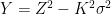
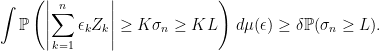
![\displaystyle \setlength\arraycolsep{2pt} \begin{array}{rl} \displaystyle{\mathbb P}(\vert Z\vert>K\sigma)&\displaystyle\ge{\mathbb E}[Z^2-K^2\sigma^2]^2/{\mathbb E}[(Z^2-K^2\sigma^2)^2]\smallskip\\ &\displaystyle=\sigma^4(1-K^2)^2/({\mathbb E}[Z^4]-2K^2\sigma^4+K^4\sigma^4)\smallskip\\ &\displaystyle\ge (1-K^2)^2/(3-2K^2+K^4) \end{array}](https://s0.wp.com/latex.php?latex=%5Cdisplaystyle++%5Csetlength%5Carraycolsep%7B2pt%7D+%5Cbegin%7Barray%7D%7Brl%7D+%5Cdisplaystyle%7B%5Cmathbb+P%7D%28%5Cvert+Z%5Cvert%3EK%5Csigma%29%26%5Cdisplaystyle%5Cge%7B%5Cmathbb+E%7D%5BZ%5E2-K%5E2%5Csigma%5E2%5D%5E2%2F%7B%5Cmathbb+E%7D%5B%28Z%5E2-K%5E2%5Csigma%5E2%29%5E2%5D%5Csmallskip%5C%5C+%26%5Cdisplaystyle%3D%5Csigma%5E4%281-K%5E2%29%5E2%2F%28%7B%5Cmathbb+E%7D%5BZ%5E4%5D-2K%5E2%5Csigma%5E4%2BK%5E4%5Csigma%5E4%29%5Csmallskip%5C%5C+%26%5Cdisplaystyle%5Cge+%281-K%5E2%29%5E2%2F%283-2K%5E2%2BK%5E4%29+%5Cend%7Barray%7D+&bg=ffffff&fg=000000&s=0&c=20201002) |
and the result follows by taking 
Lemma 3 can be used to give the following result concerning sums of random variables.
Lemma 4 Let
be a sequence of random variables such that the set
is bounded in probability. Then,
is almost surely finite. In particular,
almost surely and, hence, also in probability.

Proof: Set 


 |
Now, choose a positive constant L, multiply both sides by 

 |
(7) |
For any 

 |
Now, let n increase to infinity,
 |
Finally, as 
This result shows that, in the case where V is a space
Theorem 5 Let
be a probability space. Then, a linear map
extends to an
- For any sequence
Proof: It just needs to be shown then the second condition of Theorem 2 is satisfied. First, note that the condition of the theorem is strong enough to ensure that the set
 |
is bounded in probability. This follows from the sequential characterization of boundedness — if 

Now consider a sequence 


Proof of the existence of the stochastic integral
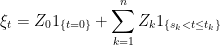
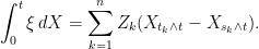
Throughout this section, it is assumed that X is a cadlag adapted process and that the set in (3) is bounded in probability. Fixing a time t, define 
Lemma 6 If
Proof: By definition of ucp convergence, 


By extension of continuous linear functions, this allows us to uniquely extend 


Every uniformly bounded, continuous and adapted process
 |
converge uniformly on compacts to
Lemma 7
.
Proof: As noted above,
Suppose that a sequence of nonnegative processes 

![{C_n\equiv\{s\in[0,T]\colon\xi^n_{s}(\omega)\ge\epsilon\}}](https://s0.wp.com/latex.php?latex=%7BC_n%5Cequiv%5C%7Bs%5Cin%5B0%2CT%5D%5Ccolon%5Cxi%5En_%7Bs%7D%28%5Comega%29%5Cge%5Cepsilon%5C%7D%7D&bg=ffffff&fg=000000&s=0&c=20201002)


Theorem 5 can now be applied to find an
Choosing 
 |
Approximating uniformly by the elementary processes 
 |
where 
 |
where 


Notes
The definition I gave for a semimartingale as being any cadlag adapted process with respect to which the stochastic integral is well-defined differs somewhat from the `classical’ definition. Historically, semimartingales have been defined as processes which can be decomposed into the sum of a local martingale and an FV process. Stochastic integration was developed with respect to such processes using generalizations of the Ito isometry applied to locally square integrable martingales. It was later shown, by the Bichteler-Dellacherie theorem, that any process satisfying the conditions of Theorem 1 above does have such a decomposition. So, the classical semimartingale definition does indeed agree with one given in these notes.
A different approach is used here, because it is possible to approach subjects such as Ito’s lemma and stochastic differential equations immediately in their full generality, without first developing a lot of technical machinery. Also, the proof given in this post that stochastic integration can be performed with respect to all processes satisfying the conditions of Theorem 1 is much, much more direct than the classical one. For example, it should be clear that the hypothesis that X is adapted can be dropped altogether, as it wasn’t even used anywhere above. Furthermore, right-continuity is only required right at the end to ensure that the constructed integral agrees with the formula for elementary processes.
Later authors have used a closer approach to the one in these notes. For example, Protter (Stochastic Integration and Differential Equations) gives two definitions of semimartingales. Both the classical definition, and the one given by Theorem 1 above are provided. Using this newer semimartingale definition, he is able to derive the stochastic integral for integrands which are L-processes (left continuous with right limits) using continuity under ucp convergence as stated in Lemma 6 above. This is enough for many applications, such as Ito’s lemma. However, he doesn’t extend the integral to arbitrary predictable integrands directly, instead relying on the Bichteler-Dellacherie theorem to show that the classical and newer semimartingale definitions agree. Then, for the full development of the integral, techniques closer to the standard ones were used.
The only author I am aware of who has developed stochastic calculus without relying on the classical definition is Bichteler (Stochastic Integration with Jumps), where a semimartingale was defined as any process satisfying the conditions of Theorem 1, and the integral was developed directly from this. This method seems to date back to a 1981 paper by the same author (Stochastic Integration and Lp-Theory of Semimartingales). It is from his treatment of stochastic integration where the idea of using the Khintchine inequality (Lemma 3) to simplify the construction of the integral was obtained. This allowed us to remove the second condition in Theorem 2. There are other methods of proving that the integral satisfies this property, but the use of the Khintchine inequality shows that it is much more general, applying to arbitrary 


Hello. First, I must thank you for your great blog! I have read them (multiple times! they are sometimes not easy to follow…) and learned a lot from them.
I have a question regarding the proof of Theorem 5. In the proof you prove that, given a sequence such that
  , then
  converges to 0 in probability. From here you imply the boundedness in probability of the image of the unit ball under the (continuous) linear operator, by invoking the sequential characterization of boundedness. However, if I understand it correctly, that characterization requires convergence to 0 of all, not just some, sequences of the form
  , with
  . For real numbers it is obvious, since the sequence
  satisfies that
  converges to zero but is not bounded.
On the other hand, for the particular case at hand (images of bounded, adapted, continuous processes) boundedness follows from the continuity under uniform convergence, which is guaranteed by continuity under UCP convergence.
Sorry, I did not answer this comment when it was posted. The sequential characterisation of boundedness applies here because is an arbitrary sequence bounded by 1. Let
  be any sequence of positive reals and S be a set of random variables. If
  in probability for every sequence
  , then S is bounded in probability.
Instead of working with $V = L^0$, could you immediately work with $V$ being the space of adapted right-continuous processes under the ucp topology and construct the integral not for each $t \geq 0$ but immediately as a process on $[0,\infty)$?
I think you probably could, using ucp convergence.
I have a small question.
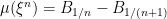
In the second part of the post, under the heading “Proof of the existence of stochastic integral”, you mentioned that $latex{\mu(\xi)}$ is continuous under the topology of uniform convergence for $latex\xi$ and this can be strengthened to uniform convergence on compacts in probability.
I didn’t get how this is possible.
Thanks a lot for the posts. They are extremely helpful.