Rademacher Concentration Inequalities

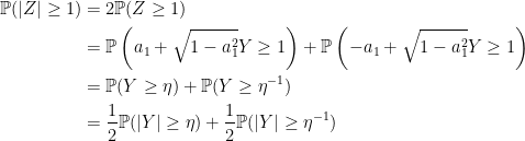
Concentration inequalities place lower bounds on the probability of a random variable being close to a given value. Typically, they will state something along the lines that a variable Z is within a distance x of value μ with probability at least p,

(1)

Although such statements can be made in more general topological spaces, I only consider real valued random variables here. Clearly, (1) is the same as saying that Z is greater than distance x from μ with probability no more than q = 1 – p. We can express concentration inequalities either way round, depending on what is convenient. Also, the inequality signs in expressions such as (1) may or may not be strict. A very simple example is Markov’s inequality,

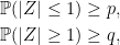
In the other direction, we also encounter anti-concentration inequalities, which place lower bounds on on the probability of a random variable being at least some distance from a specified value, so take the form

(2)

An example is the Paley-Zygmund inequality,

which holds for all 0 ≤ x ≤ 𝔼|Z|.

While the examples given above of the Markov and Paley-Zygmund inequalities are very general, applying whenever the required moments exist, they are also rather weak. For restricted classes of random variables much stronger bounds can often be obtained. Here, I will be concerned with optimal concentration and anti-concentration bounds for Rademacher sums. Recall that these are of the form

for IID random variables X = (X₁, X₂, …) with the Rademacher distribution, ℙ(X_n = 1) = ℙ(X_n = -1) = 1/2, and a = (a₁, a₂, …) is a square-summable sequence. This sum converges to a limit with zero mean and variance

I discussed such sums at length in the posts on Rademacher series and the Khintchine inequality, and have been planning on making this follow-up post ever since. In fact, the L⁰ Khintchine inequality was effectively the same thing as an anti-concentration bound. It was far from optimal as presented there, and relied on the rather inefficient Paley-Zygmund inequality for the proof. Recently, though, a paper was posted on arXiv claiming to confirm conjectured optimal anti-concentration bounds which I had previous mentioned on mathoverflow. See Tight lower bounds for anti-concentration of Rademacher sums and Tomaszewski’s counterpart problem by Lawrence Hollom and Julien Portier.

While the form of the tight Rademacher concentration and anti-concentration bounds may seem surprising at first, being piecewise constant and jumping between rather arbitrary looking rational values at seemingly arbitrary points, I will explain why this is so. It is actually rather interesting and has been a source of conjectures over the past few decades, some of which have now been proved and some which remain open. Actually, as I will explain, many tight bounds can be proven in principle by direct computation, although it would be rather numerically intensive to perform in practice. In fact, some recent results — including those of Hollom and Portier mentioned above — were solved with the aid of a computer to perform the numerical legwork.

---

Anti-Concentration Bounds

For a Rademacher sum Z of unit variance, recall from the post on the Khintchine inequality that the anti-concentration bound

(3)

holds for all non-negative x ≤ 1. This followed from Payley-Zygmund together with the simple Khintchine inequality 𝔼[Z²] ≤ 3. However, this is sub-optimal and is especially bad in the limit as x increases to 1 where the bound tends to zero whereas, as we will see, the optimal bound remains strictly positive.

In the other direction if, for positive integer n, we choose coefficients a ∈ ℓ² with a_k = 1/√n for k ≤ n and zero elsewhere then, by the central limit theorem, Z = a·X tends to a standard normal distribution. as n becomes large. Hence

where Φ is the cumulative normal distribution function. So, any anti-concentration bound must be no more than this.

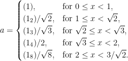
The optimal anti-concentration bounds have been open conjectures for a while, but are now proved and described by theorem 1 below, as plotted in figure 1. They are given by a piecewise constant function and, as clear from the plot, lie strictly between the simple Paley-Zymund bound and Gaussian probabilities.

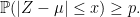
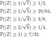
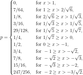
Theorem 1 The optimal lower bound p for the inequality ℙ(|Z| ≥ x) ≥ p for Rademacher sums Z of unit variance is,

At first sight, this result might seem a little strange. Why do the optimal bounds take this discrete set of values, and why does it jump at these arbitrary seeming values of x? To answer that, consider the distribution of a Rademacher sum. When all coefficients are small it approximates a standard normal and the anti-concentration probabilities approach those indicated by the ‘Gaussian bound’ in figure 1. However, these are not optimal, and the minimal probabilities are obtained at the opposite extreme with a small number n of relatively large coefficients and the remaining being zero. In this case, the distribution is finite with probabilities being multiples of 2^–n, and the bound jumps when x passes through the discrete levels.

The values of a ∈ ℓ² for which the stated bounds are achieved are not hard to find. For convenience, I use (a₁, a₂, …, a_n) to represent the sequence starting with the stated values and remaining terms being zero, a_k = 0 for k > n. Also, if c is a numeral than c_k will denote repeating this value k times.

Lemma 2 The optimal lower bound stated by theorem 1 for Rademacher sum Z = a·X is achieved with

This is straightforward to verify by simply counting the number of sign values of (X₁, |, X_n) for which |a·X| ≥ x and multiplying by 2^–n. It does however show that it is impossible to do better than theorem 1 so that, if the bounds hold, they must be optimal. Also, as ℙ(|Z| ≥ x) is decreasing in x, to establish the result it is sufficient to show that the bounds hold at the values of x where it jumps. This reduces theorem 1 to the following finite set of inequalities.

Theorem 3 A Rademacher sum Z of unit variance satisfies,

The last of these has been an open conjecture for years since it was mentioned in a 1996 paper by Oleszkiewicz. I asked about the first one in a 2021 mathoverflow question, and also mentioned the finite set of values x at which the optimal bound jumps, hinting at the full set of inequalities, which was the desired goal. Finally, in 2023, a preprint appeared on arXiv claiming to prove all of these. While I have not completely verified the proof and the computer programs used myself, it does look likely to be correct.

Although the bounds given above are all for anti-concentration about 0, a simple trick shows that they will also hold about any real value.

Lemma 4 Suppose that the inequality ℙ(|Z| ≥ x) ≥ p holds for all Rademacher sums Z of unit variance. Then the anti-concentration bound

also holds about every value μ.

Proof: If Z = a·X and, independently, Y is a Rademacher random variable, then Z + μY is a Rademacher sum of variance 1 + μ². This follows from the fact that it has the same distribution as b·X where b = (μ, a₁, a₂, …). So,

By symmetry of the distribution of Z, both probabilities on the right are equal giving,

implying the result. ⬜

You have probably noted already, that all of the coefficients described in lemma 2 are of the form (1_n)/√n. That is, they are a finite a sequence of equal values with the remaining terms being zero. In fact, it has been conjectured that all optimal concentration and anti-concentration bounds (about 0) for Rademacher sums can be attained in this way. This is attributed to Edelman dating back to private communications in 1991. If true, it would turn the process of finding and proving such optimal bounds into a straightforward calculation but, unfortunately, in 2012, the conjecture was shown to be false by Pinelis for some concentration inequalities.

Before moving on, let’s mention how such bounds can be discovered in the first place. Running a computer simulation for randomly chosen finite sequences of coefficients very quickly converges on the optimal values. As soon as we randomly select values close to those given by lemma 2, we obtain the exact bounds and any further simulations only serve to verify that these hold. Running additional simulations with coefficients chosen randomly in the neighbourhood of points where the bound is attained, and near certain ‘critical’ values where the bound looks close to being broken, further strengthens the belief that they are indeed optimal. At least, this is how I originally found them before asking the mathoverflow question, although this is still far from a proof.

---

Concentration Bounds

For random variables with zero mean and unit variance, Markov’s (or Chebyshev’s) inequality directly gives

Figure 2 plots conjectured optimal upper bounds for ℙ(|Z| > x) for unit variance Rademacher sums, which we see lie between the simple Markov bound and the Gaussian probabilities.

To be consistent with the presentation above, it will be convenient to work with concentration bounds of the form ℙ(|Z| ≥ x) ≤ p,. Clearly, this is the same as looking at upper bounds for ℙ(|Z| > x) by exchanging p with 1 – p. While optimal bounds are not fully known, for small values of x they are conjectured to be as in figure 2.

Conjecture 5 The optimal lower bound p for the inequality ℙ(|Z| ≤ x) ≥ p for Rademacher sums Z of unit variance is,

The case with x = 1 is especially interesting,

This was conjectured back in 1986 in the American Mathematical Monthly article ‘Any Answers Anent These Analytical Enigmas?‘, and attributed to Bogusłav Tomaszewski. It has become known as Tomaszewski’s conjecture, with many partial proofs and ever-improving suboptimal bounds produced over the years. It was eventually proved in 2020 by Keller and Klein in the paper ‘Proof of Tomaszewski’s Conjecture on Randomly Signed Sums‘. The remaining bounds for x ≥ √2 above are still open, with the conjectured values appearing in the same 2023 paper of Hollom & Portier that proved the anti-concentration inequalities.

In contrast to anti-concentration inequalities which become trivial for x > 1, the concentration bounds are always strictly between 0 and 1 for all x > 1. Furthermore, as indicated in figure 2, they are sandwiched between between the values from Markov’s inequality and the Gaussian probabilities, both of which are strictly increasing towards 1. This means that the optimal Rademacher concentration bounds will never be eventually constant for large x, so it is unlikely that simple formulas covering all x > 0. There are, however, studies on the asymptotic behaviour of these tail bounds. For example, in the 2010 paper ‘An asymptotically Gaussian bound on the Rademacher tails‘, Pinelis establishes a bound which is asymptotic to the Gaussian probabilities;

for standard normal Y and constant c. Such asymptotic approximations are not the focus of this post, however. Instead, we look at exact optimal solutions for small values of x.

As with the anti-concentration case, finding Rademacher sums achieving the optimal bounds of conjecture 5 is not difficult. The following can be checked by direct calculation.

Lemma 6 The optimal lower bound stated by conjecture 5 for Rademacher sum Z = a·X is achieved with

As a result, if the conjectured bounds do hold, then they are necessarily optimal. Also, as ℙ(|Z| ≤ x) is increasing, it is sufficient to prove that they hold at the x values where they are discontinuous. Hence, conjecture 5 is equivalent to the following finite set of inequalities.

Conjecture 7 A Rademacher sum Z of unit variance satisfies,

The proof of Lemma 4 also carries across almost unchanged to the current situation (reversing inequalities where necessary), giving concentration bounds about an arbitrary point μ.

Lemma 8 Suppose that the inequality ℙ(|Z| ≤ x) ≥ p holds for all Rademacher sums Z of unit variance. Then the concentration bound

also holds about every value μ.

Here, we cannot remove the factor of √1 + μ² since it would reduce the probability so that the bound may not hold. This is to be expected. Rademacher sums are concentrated about zero, and concentration bounds about other points must necessarily be weaker.

---

Combined Concentration and Anti-Concentration Bounds

Since the distribution of a Rademacher sum Z is symmetric, the concentration and anti-concentration probabilities convert directly to its cumulative distribution function,

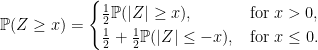So, the inequalities stated in theorem 1 and conjecture 5 can be combined into a single set of bounds for the distribution function.

Conjecture 9 The optimal lower bound p for the inequality ℙ(Z ≥ x) ≥ p for Rademacher sums Z of unit variance is,

As already discussed, most of these have been open conjectures for some time but, recently, all cases with x > -√2 have now been proved. Considering inequalities in this form will be convenient since they generate both concentration and anti-concentration bounds for x < 0 and x > 0 respectively.

---

Berry–Esseen

A Rademacher sum Z = a·X of unit variance is close to the normal distribution when all coefficients are small. While this follows from considering the characteristic function, good quantitative bounds are very useful, which is where the Berry–Esseen theorem comes in. For unit variance Rademacher sums this states that

for a constant C, where Φ is the standard normal distribution function. Whilst ever smaller values of the constant have been proved over the years, C = 0.56 was shown to be valid by Shevstova in the 2010 paper ‘An improvement of convergence rate estimates in the Lyapunov theorem‘.

As the distribution of Z does not depend on the sign or ordering of the coefficients a_i, without loss of generality they can be assumed to be nonnegative and decreasing. In this case, ‖a‖₁ = a₁ and Berry–Esseen can conveniently be written as

Since the characteristic function of Rademacher sums is relatively straightforward, there are much better approximations available. A method due to Prawitz gives bounds on the distribution function based on partial knowledge of the characteristic function. In their 2020 paper, Keller and Klein applied this to Rademacher sums to obtain an alternative to Berry–Esseen, with the Ca₁ term replaced by a rather complicated but much more accurate integral expression. I will not go over the details here, but note that results following from the use of Berry–Esseen in this post can be strengthened with the use of such improved bounds.

---

Baby Steps: First Nontrivial Bounds

Consider the inequalities

for Z = a·X a unit variance Rademacher sum. As stated above, the optimal values are p = 1/2 and q = 7/32.However, to get started, how to prove any bound with p and q strictly positive? The example with a = (1) has ℙ(|Z|< 1) and ℙ(|Z| > 1) both equal to 0, so any positive values of p or q get very close to failure.

A common approach is to assume w.l.o.g. that the coefficients a_i are nonnegative and decreasing, and use different approaches for small and large values of a₁. For small values, Berry–Esseen gives

For small values of a₁, the left side bound is less than 1 and the right side is strictly positive.

For larger values of a₁ < 1, decompose

where Y = (1 - a₁²)^-1/2Σ_n≥2a_nX_n is a unit variance Rademacher sum independent of X₁.

(4)

with η = √(1 - a₁)/(1 + a₁). For the concentration bound, Markov’s inequality bounds the second term on the right hand side from above,

For the anti-concentration bound, the Paley-Zygmund inequality (3) bounds the first term on the right of (4),

So, using Berry-Esseen for a₁ below a threshold value and the second approach above it gives a non-trivial bound. Plugging in the numbers for a threshold of 0.369 in the concentration bound and 0.258 in the anti-concentration one gives

Aint much, but its honest work.

---

Compactness of the Domain

The distribution of a Rademacher sum Z = a·X does not depend on the signs or on the order of the coefficients a_i. Hence, by flipping their signs and reordering if necessary, we can assume that they are nonnegative and decreasing,

(5)

This is a fairly standard step in many proofs involving Rademacher sums in the literature. It not only reduces the size of the space, but also has the benefit of placing the most impactful coefficients first. In fact, it removes all degeneracy from the representation since, now, it gives a one-to-one map from the coefficients to Rademacher sum distributions.

The space of Rademacher sums is not complete. Specifically, for coefficients a = (1_n)/√n then, by the central limit theorem, a·X tends to a standard normal as n goes to infinity, which is not itself a Rademacher sum. The completion under convergence in law can be shown to be that of independent sums of Rademacher sums and centered normal distributions. I will refer to such as completed Rademacher sums. For any a ∈ ℓ², with ‖a‖₂ ≤ 1, write

(6)

for an IID sequence X = (X₁, X₂, …) of Rademacher random variables and, independently, a standard normal X_∞.

Now, I will use ℓ²_1,d to denote the space of a ∈ ℓ² with ‖a‖₂ ≤ 1 and decreasing nonnegative coefficients (5), equipped with the product topology (i.e., pointwise convergence). This is compact, and the map a ↦ a·X is a homeomorphism from ℓ²_1,d to the completed Rademacher sum distributions of unit norm. In particular, this shows that the completed Rademacher sums of unit variance are compact under convergence in law, and hence the unit norm Rademacher sums are relatively compact.

Compactness has many theoretical benefits.Suppose that we want to prove an inequality of the form

(7)

Given any choice of a ∈ ℓ²_1,d, we can directly compute the probability as accurately as we like and verify (7) — if indeed it does hold. By continuity of the map a ↦ S_a, this proves that (7) also holds in a neighbourhood of a. This makes use of the fact that, as the probability uses a strict inequality, it is lower semicontinuous. By compactness, the whole space can be covered by finitely many such neighbourhoods and, so, to prove that (7) holds for all unit variance Rademacher sums, it is only necessary to verify that it holds for a finite set of coefficients a ∈ ℓ²_1,d.

Unfortunately, bounds such as (7) are not optimal. If we try to improve it by making x and p as large as possible, then the inequalities will not be strict and, instead, we need to prove

(8)

The compactness argument above no longer holds since, even if we show that (8) holds for some a ∈ ℓ²_1,d then it does not automatically follow that it also holds in a neighbourhood of this. Much of the aim of this post is to show that, with some assumptions and special treatment at certain ‘critical’ points, we can in fact infer that (8) extends to a neighbourhood and so a proof of the optimal bound does indeed follow from verifying it at a finite number of points. This is in theory — I am not giving full proofs here, and it could potentially involve validating the bound at a lot of points. Notably, the known proofs of the optimal bounds found so far do involve computer assistance.

What does a neighbourhood of a point a ∈ ℓ²_1,d look like? Well, we can define a basis of neighbourhoods U_δ(a) for strictly positive finite sequences δ = (δ₁, …, δ_N). This consists of b ∈ ℓ²_1,d such that |b_i – a_i|< δ_i for i ≤ N. Such sets only involve the first N components of a so, in any completed proof, we just need to refer to sequences whose first N components are within some range. Furthermore, it is sufficient to only look at standard Rademacher sums b·X for ‖b‖₂ = 1 (without the Gaussian term), since these are dense. In fact, it is sufficient to only consider finite Rademacher sums.

Many proofs of bounds (either optimal or not) are, in fact, largely structured like this, breaking the domain down into a finite number of such neighbourhoods. My non-optimal proof above is of this form, although it only involved looking at two subsets of the domain based on the value of a₁. Proofs of optimal bounds involve looking at neighbourhoods defined by more terms (N > 1). The use of completed sums is my own consideration to describe how, theoretically, compactness can result in rigorous proofs by looking at neighbourhoods of a finite set of points.

---

Finite Rademacher Sums

Proving concentration inequalities reduces to proving them for finite length Rademacher sums,

The results for infinite sequences follow by allowing n to go to infinity. For now, consider sums of a fixed finite length.This makes proving concentration bounds much more tractible. However, the methods used for bounded length sums get computationally very difficult very quickly as n becomes large, and do not seem to lead to proofs for infinite or unbounded length sums. They do, however, provide some evidence for the bounds and give confidence that they actually hold in general.

Computing the probability that Z ≥ x amounts to counting the number of sign choices for which

and multiplying by 2^–n. Inequality ℙ(Z ≥ x) ≥ 2^–nc amounts to showing that at least c choices of signs gives a sum equal to or greater than x. This can be expressed as a system of linear inequalities — for some collection of c sign choices, the corresponding signed sums of the coefficients are all greater than x. Admittedly, this gives rather a lot of inequalities, especially if n is large. Showing that it holds for all coefficients with unit sum of squares amounts to showing that, on the complement of the domain, defined by linear inequalities, the sum of squares of coefficients does not attain the value 1. This reduces to a quadratic programming problem, which can be solved entirely systematically. This is in theory. In practice, the complexity grows very quickly in the number n of coefficients, and quickly becomes impractical.

Although proving (anti-)concentration bounds for finite Rademacher sums becomes unwieldy even for relatively small n, algebraic tricks can often be used to obtain short proofs. For example, Oleszkiewicz gave a short proof that ℙ(Z ≥ 1) ≥ 7/64 for sums of length 6 in the 1996 paper ‘On the Stein Property of Rademacher Sequences‘. I present a proof here along similar lines.

We first note that changing the signs and ordering of the coefficients does not affect the distribution of the Rademacher sum. Without loss of generality, then, they can be assumed to be nonnegative and decreasing (5). Next, I call a sequence of ‘+’ and ‘-‘ signs good if the coefficients summed with these signs, in order, gives a result which is greater than or equal to 1. For example, (++-+-+) being good is just shorthand for

With this notation, and assuming the sum of squares of the coefficients equals 1, we can prove the following.

Lemma 10 At least one of

is good.

Before proving this result, I explain how it implies the claimed anti-concentration bound. As the coefficients a_i are nonnegative and decreasing, changing a ‘-‘ sign into ‘+’ or shifting it to the right only increases the value of the sum, so the sequence is still good. So, the second sequence stated in the lemma actually results in 8 good sequences,

Hence, ℙ(Z ≥ 1) ≥ 8/64 for this case. In the same way, each of the other two possibilities in lemma 10 generates 7 good sign sequences. So, ℙ(Z ≥ 1) ≥ 7/64 as claimed.

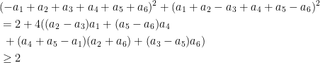
Proof of lemma 10: If a₁ ≥ a₄ + a₅ then a little algebraic rearranging gives,

The inequality follows from the fact that a_i are nonnegative and decreasing so that each of the bracketed terms on the second line are nonnegative. Hence, at least one of the squares in the first line is greater than or equal to 1, showing that (++-++-) or (+++- -+) is good.

Alternatively, if a₁ ≤ a₄ + a₅, the same argument gives

so that (-+++++) or (++-++-) is good. ⬜

While studying Rademacher sums of fixed finite length can hint at the more general situation and give us some confidence in the bounds, it does not seem to lead on to proofs of concentration and anti-concentration inequalities for infinite sums or sums of unrestricted length.

---

Decomposing the Sum

A unit variance Rademacher sum Z = a·X can be decomposed into its first n terms plus the remainder

(9)

where I have set

So Z_n and Y_n are independent unit variance Rademacher sums, with Z_n of length n and taking the 2ⁿ values ±a₁ + ⋯±a_n with equal probability. This is a commonly used decomposition, since the distribution of Z_n has such a simple and discrete distribution, and Y_n has a small contribution to the distribution when σ_n is small, as will be the case for large enough n. It is undefined for the edge case with coefficients equal to 0 after the first n terms, since it involves dividing by σ_n = 0 but, here, Y_n can be set to whatever we like. In particular, this can be used to directly prove bounds like ℙ(Z > x) > p simply by choosing n large enough and verifying that it holds for Z_n.

Rearranging,

(10)

The conditional probability can be bounded using known, possibly suboptimal bounds for Y_n. Writing out the expectation more explicitly,

(11)

where z ranges of the 2ⁿ values that Z_n can take (with multiplicity). The probabilities on the right hand side involving Y_n can be replaced by already-known bounds in order to generate new ones. A very simple bound which can be useful is

when z ≥ x, which is just a consequence of the symmetry of Y_n. For example, it very easily gives the following simple anti-concentration inequality,

Lemma 11 The bound ℙ(|Z| ≥ x) ≥ 2^–n holds whenever a₁ + ⋯+a_n ≥ x.

Proof: By (11),

The right hand side includes the term with z = a₁ + ⋯+a_n ≥ x, which has a probability of at least 1/2, giving the result. ⬜

By combining with the Berry–Esseen bound, lemma 11 can be used to derive an unconditional concentration inequality.

Lemma 12 ℙ(|Z| ≥ 0.26) ≥ 1/2.

Proof: For a₁ ≥ x = 0.26 the inequality holds by lemma 11, so suppose that a₁ < x. Berry–Esseen gives

as required. ⬜

The claim is that this still holds with 1/√7 ≈ 0.38 in place of 0.26 but, for such a simple proof, lemma 12 does quite well. More advanced applications of (11) rely on bounds on sums of more than one probability on the right-hand-side, rather than bounding each term individually. A simple example is

(12)

whenever (z + z′)/2 ≥ x. This again makes use of symmetry, since the left hand side is

which is at least 1 as x – z ≤ z′-x. This means that we can bound the right hand side of (11) by pairing together levels which average more than x. I do this further below when explaining how to handle critical points.

An alternative rearrangement of (11) gives

which says that the probability that Z ≥ x is the probability for Z_n plus the probability that Z_i increases from Z_n < x to above x and minus the probability of dropping from Z_n ≥ x to below x. Expanding out the expectation as a sum again,

(13)

A specific case where this is useful is where ℙ(Z_n ≥ x) is equal to the optimal bound. In that eventuality (13) reduces to showing that

(14)

Yet another approach is to find a bound which works for any value of Y_n. Directly from the decomposition (9),

(15)

where the infimum is taken over all real y. Bounding the right hand side for any specified coefficients (a₁, …, a_n) is straightforward, as Z_n has a finite distribution. A well-known result of Erdös generalizes lemma 11.

Lemma 13 Suppose that a_m + a_m+1 + ⋯+a_n ≥ x for some m ≤ n. Then,

(16)

where c is the sum of the m smallest binomial coefficients of the form over 0 ≤ i ≤ n.

Proof: For any subset U of {1, …, n} let z_U denote the sum of the coefficients a_i over i ≤ n, with a minus sign for each i ∈ U. Then, for real y,

where consists of sets U for which |z_U – y|< x. For any pair of sets U ⊆ V in then V ∖ U must have no more than n – m elements. To see why, note that z_U – z_V is twice the sum of a_i for i in V ∖ U. By the condition of the lemma, if it had size more than n – m then z_U ≥ z_V + 2x contradicting the fact that .

From theorem 4 of the paper On a lemma of Littlewood and Offord by Erdös, is no more than the sum of the n – m + 1 largest binomial coefficients. So,

and the result follows from (15). ⬜

For an example application, which is useful for the optimal anti-concentration bound with x = 1;

Lemma 14 If a₃ + a₄ + a₅ ≥ x then ℙ(|Z| ≥ x) ≥ 7/32.

Proof: Simply apply lemma 13 for m = 3 and n = 5, noting that the 3 smallest binomial coefficients are 1, 1, 5 for i = 0, 5, 1 respectively. ⬜

---

Splitting the Domain

Recall from above that we aim to prove bounds ℙ(S_a ≥ x) ≥ p for all a in the domain ℓ²_1,d and, by compactness, it is sufficient to be able to do this in a neighbourhood of any point a ∈ ℓ²_1,d. This domain can be split into three separate regions of varying difficulty.

Subspace A: ℙ(S_a > x) > p.
Subspace B: ℙ(S_a > x) = p.
Subspace C: ℙ(S_a > x) < p.

Subspace A is the easiest. Due to continuity of the map a ↦ S_a, if the inequality holds at a point then it automatically holds in some neighbourhood. Of course, if performing this in practice, then it will be necessary to explicitly compute a modulus of continuity or similar. Recall that continuity was proved by showing that the characteristic function of S_a depends continuously on a. Likewise, explicitly computed bounds based on the characteristic function can be used here, such as the method of Prawitz used by Keller and Klein. Combining with additional tricks can further reduce the computational work required. However, as this case is easily handled in theory, I will say nothing further about subspace A.

Subspace B is a bit more difficult to handle, and relying on continuity is not enough. Certainly there are points where the optimal bounds are attained, as demonstrated in lemmas 2 and 6. By continuity alone, we cannot rule out the possibility that ℙ(S_a ≥ x) drops below p under arbitrarily small bumps to a. As I show below, under an additional assumption which seems to hold in reality, it is possible to show that this does not happen and a neighbourhood can be computed in which the bound holds.

Subspace C is most difficult. I will refer to these as critical points and it seems necessary to use rather ad-hoc methods on a case-by-case basis. However, there are only finitely many critical points which can be dealt with explicitly.

---

Critical Points

For a bound ℙ(S_a ≥ x) ≥ p, I refer to a ∈ ℓ²_1,d for which the strict inequality ℙ(Z > x) is less than p as critical. In that case, assuming that the bound does indeed hold,

This can only happen if a only has finitely many nonzero terms. Also, it can be shown that any limit point of critical values in ℓ²_1,d satisfies ℙ(S_a > x) = p, which is in subspace B according to the classification above. As I will show, under an assumption, the inequality ℙ(S_a > x) ≥ p holds in the neighbourhood of points of subspace B, they cannot be limits of critical points. Hence, for any given values of x and p, there can only be finitely many critical points.

It is not difficult to find critical points by manually looking for them. Also, the proofs of anti-concentration inequalities by Keller & Klein and by Hollom & Portier,explicitly handle these values, so can be found in the papers. Figure 4 lists the critical points for some values of x and p. Also shown are the probabilities ℙ(S_a ≥ x) and ℙ(S_a > x) along with their values to several decimal places for easy comparison.

x	p		a	ℙ(Sa ≥ x)		ℙ(Sa > x)
1	7/64	0.109	(1)	1/2	0.50	0	0.000
1	7/64	0.109	(14)/2	5/24	0.31	1/24	0.063
1	7/64	0.109	(19)/3	65/28	0.25	23/28	0.090
1	7/64	0.109	(116)/4	14893/216	0.23	6885/216	0.105
1	7/64	0.109	(2,15)/3	17/26	0.27	3/25	0.094
1	7/64	0.109	(2,112)/4	1885/213	0.23	873/213	0.107
1	7/64	0.109	(22,18)/4	119/29	0.23	111/210	0.108
2/√6	1/8	0.125	(16)/√6	11/25	0.34	7/26	0.109
1/√3	3/16	0.188	(13)/√3	1/2	0.50	1/23	0.125
1/√5	29/128	0.227	(15)/√5	1/2	0.50	3/24	0.188
1/√7	1/4	0.250	(17)/√7	1/2	0.50	29/27	0.227
-1	3/4	0.750	(1)	1	1.00	1/2	0.500
-1	3/4	0.750	(14)/2	15/24	0.94	11/24	0.688
-1	3/4	0.750	(19)/3	233/28	0.91	191/28	0.746

Note that for any unit variance Rademacher sum Y independent of S_a, then Z = √1 - ϵ²S_a + ϵY is also a Rademacher sum for any ϵ > 0. Also, expanding to second order for small ϵ,

(17)

Consider the case where Y is distributed as b·X for b = (1₂)/√2. This has Y = √2 with probability 1/4 otherwise, Y ≤ 0. So, for sufficiently small ϵ, when S_a > 0 we have Y ≥ S_a with probability 1/4,

This proves the following.

Lemma 15 Assume the bound ℙ(S_a ≥ x) ≥ p holds for all a ∈ ℓ²_1,d and some x > 0. If a is a critical point then

(18)

Checking figure 4, it can be seen that this is indeed the case at critical points with x > 0. The argument above does not apply for x < 0 since, when S_a < 0, the term in parenthesis on the right of (17) will be positive rather than negative for Y = 0. Indeed, checking the critical point for x = 1, (18) fails. Instead, we obtain a weaker result which holds for all x.

Lemma 16 Assume the bound ℙ(S_a ≥ x) ≥ p holds for all a ∈ ℓ²_1,d. If a is a critical point then

(19)

This again follows from (17) where, now, we suppose that Y is Rademacher, ℙ(Y = ±1) = 1/2. Then, for small ϵ, the term in parentheses is positive when Y = 1 and negative when Y = -1.

While the results stated in lemmas 15 and 16 are necessary in order for the bound to hold, the converse is not true. We cannot simply deduce that the bound holds everywhere from the observation that ℙ(S_a = x) is sufficiently large.

How can we prove that the proposed bound does indeed hold in a neighbourhood of a critical point a? For anti-concentration inequalities at least, the methods described above in decomposing the sum are sufficient. For a fixed number n of initial non-zero coefficients, write the probability using (11)

(20)

where z ranges over the 2ⁿ values ±a₁±⋯±a_n. Individual terms, or pairs of terms, can be bounded using,

(21)

The 0.26 term comes from lemma 12. We know that the improved value 1/√7 ≈ 0.37 could be used once the anti-concentration bounds have already been established, but this is not important here.

To demonstrate the idea, consider a neighbourhood of the critical point (1₄)/2 for the bound ℙ(Z ≥ 1) ≥ 7/64. We have,

for some small bumps δ_i which can be either positive or negative, but are in decreasing order. The values that z ranges over in (20) includes

As (z₀ + z₁)/2 ≈ 3/2 > 1 for small δ, the terms in (20) involving these values of z contribute a total of 2^-4 = 4/64 to the probability. It remains to show that the other terms contribute at least 3/64. The case with a₁ + a₂ ≥ 1 is already dealt with by lemma 11, showing that ℙ(Z ≥ 1) ≥ 1/8, so consider a₁ + a₂ ≤ 1. This corresponds to δ₁ + δ₂ ≤ 0 and, as δ_i are decreasing, shows that δ₂ ≤ 0 and the absolute values |δ_i| are increasing. Hence,

So σ₄ is at least √|δ₄|, to leading order, which will be significantly greater than x – z_i = O(δ). Using (21) then, the terms in (20) involving z_i for i = 2, 3, 4 each contribute at least 2^-4(1/4) = 1/64 to the probability, giving a total probability of at least 7/64 as required. This demonstrates the idea, but to see precise calculations of neighbourhoods of all of the critical points of anti-concentration bounds, see the paper by Hollom & Portier.

The method demonstrated for anti-concentration bounds are a bit too weak to handle concentration inequalities. On their own, the bounds (21) can never contribute more than 1/2 to the total probability. For ℙ(Z ≥ x) with negative x, this is not good enough. In the Keller & Klein paper, they need to handle the neighbourhood of the critical point at a = (1) when proving Tomaszewski’s conjecture that ℙ(|Z| ≤ 1) ≥ 1/2 or, equivalently, ℙ(Z ≥ -1) ≥ 3/4. They manage this by using an inductive proof based on a stopping-time argument to handle a₁ + a₂ ≥ 1 and, then, use ‘local inequalities’ (comparing probabilities of being in different intervals using, effectively, the reflection principle) to handle a₁ + a₂ < 1 and a₁ close to 1.

---

Equality Case

I finally look at the equality case,

(22)

corresponding to subspace B above. For fixed values of x and p, if equality occurs then we need to find a neighbourhood of a in which the bound holds. We already know that equality occurs some values of a — specifically those given by lemmas 2 and 6. In these cases, Z = S_a is a finite Rademacher sum of length n with equal coefficient values. That is, a = (1_n)/√n. Then, the value of Z = ±a₁±⋯±a_n only depends on the number of negative signs. So, there is a number r ≤ n such that Z > x if and only if there are no more than r negative signs, and Z ≤ x otherwise. This implies that

For more general length n sums we can guess that the equality case occurs in the same situation occurs, and Z ≤ x whenever there are more than r minus signs. If, as usual, the coefficients are nonnegative and arranged in decreasing order this is equivalent to

For general a ∈ ℓ²_1,d we can further guess that equality only occurs if ‖a‖₂ = 1, so that there is no Gaussian term, and if the first n terms are as above, after which the partial sums Z_i never cross level x. That is,

(23)

We know that this cannot hold for all such bounds, since Pinelis showed that, for some values of x, the optimal concentration bound cannot be attained with equal coefficients. However, for now, let’s restrict to values of x where it can. Figure 5 shows these cases, and also lists a simple condition which is satisfied in the claimed equality case (23). These are necessary conditions for equality, but not sufficient. Don’t worry if it isn’t clear why each of these conditions is implied by (23), they are not obvious, but can be shown to hold.

x	p	n	r	condition
1	7/64	6	1	a3 + a4 + a5 > 1
2/√6	1/8	3	0	a1 + a2 > x
1/√3	3/16	5	1	a3 + a4 > x
1/√5	29/128	7	2	a6 + a7 > x
1/√7	1/4	2	0	a1 > x
-1	3/4	2	1	a1 + a2 > 1

I used strict inequalities in the conditions listed in figure 5. This is because we need to prove the result on an open set containing equality cases, so that it automatically includes a neighbourhood of each a ∈ ℓ²_1,d satisfying (22). It then leaves a closed subset of ℓ²_1,d, which can be handled by the brute force method using compactness.

A consequence of strict inequalities in the conditions of figure 5 is that it actually misses out one case with equality. For x = 1 and p = 7/64, there is the single point a = (2, 1₅)/3 for which a₃ + a₄ + a₅ = 1, so does not satisfy the strict inequality mentioned, but does satisfy the equality condition (22). The anti-concentration bound can be proven in a neighbourhood of this in exactly the same way as for critical points described above. In fact, in the paper of Hollom & Portier, they include this in their list of ‘hard cases’, corresponding to what I am calling critical points.

Now, note that every one of the anti-concentration bounds in figure 5 follows immediately from an application of Lemma 16 applied to the listed condition. The concentration bound (Tomaszewski’s conjecture) with x = -1 is more difficult though. Keller & Klein handle this case, with a₁ + a₂ ≥ 1, by an ingenious stopping time argument using induction. on the length of the Rademacher sum.

So far, we have seen how the equality case can be handled for specific values of the level x, which depends on finding a simple condition on the coefficients. Whether such a condition can be found for all bounds is unclear, and seems unlikely. In fact, there is also a brute-force approach which can be much as was explained above for case ‘A’ where ℙ(S_a > x) > p. This relies on one assumption — that, for the equality case it always holds that

(24)

for some x′ > x. Equivalently, there exists a nonempty interval (x, x′) on which S_a has zero probability. While it is not obvious that (24) has to hold, it does for the values of x considered above. Furthermore, it holds whenever the equality case is characterized by (23), so just considering (24) is the more general situation and is more likely to be true for other values of x.

The idea is that, when (24) holds, then the bound can be extended to a neighbourhood of a using the following inequality.

Lemma 17 For any real numbers v > u ≥ 0 and K there exists an ϵ > 0 such that

(25)

for all unit variance Rademacher sum Z and 0 ≤ σ ≤ ϵ.

Proof: Let N be the smallest positive integer such that Z_N ≥ u. Then, Z_N ≤ u + a_N ≤ u + 1. Conditioned on N, Z – Z_N is a Rademacher sum of variance no more than 1. So, by the Markov/Chebyshev inequality,

when N < ∞. Restricting to the event Z ≥ u and taking expectations,

Dividing u, v by ϵ,

and the result follows by taking ϵ small enough. ⬜

To explain how this works, first choose x^– ≤ x < x⁺ with ℙ(S_a > x^–) = p = ℙ(S_a ≥ x⁺), choosing x^– to be minimal and x⁺ to be maximal. These define a maximal interval (x^–, x⁺) on which S_a has zero probability. This implies that ‖a‖₂ = 1 so that there is no Gaussian term (6), otherwise S_a would have full support. Equivalently, S_a = a·X is a regular Rademacher sum. If the bound ℙ(S_a ≥ x) ≥ p does indeed hold everywhere, then assumption (24) has the following consequence.

Lemma 18 Suppose that (24) holds and that ℙ(S_a > x) = p. Then,

(26)

and, for all n sufficiently large that 2a_n+1 < x⁺ – x^–,

(27)

This is using decomposition (9), where Z_n is the first n terms of the Rademacher sum Z = S_a. I will not go through the proof of lemma 18, but indicate how it can be shown. If (26) was not true, then S_a can get as close to x from above as it can from below. A small bump to the coefficients can be applied to give a positive probability of S_a dropping back below x after the first n terms, contradiction the assumption that the bound holds everywhere. Next, if 2a_n < x⁺ – x^– then, for i > n, the process Z_i cannot jump past the interval (x^–, x⁺), and cannot enter it either, otherwise it would have a positive probability of remaining within the interval, so that S_a is in the interval contradicting the definition of x^–, x⁺. Hence, S^a ≥ x⁺ if and only if Z_n ≥ x⁺, implying (27).

By (27), for any b ∈ ℓ²_1,d,

If the first n terms of b agree with a, then S_b = Z_n + σ_nY for a unit variance Rademacher sum Y independent of Z_n

From (26), there exists v > u > 0 with x – u < x^– and x + v ≤ x⁺. So, for α_n = ℙ(x - u < Z_n < x),

Choosing α < ℙ(x - u < S_a < x) then α_n < α for sufficiently large n and, if σ_n is small enough, lemma 17 gives

and the bound ℙ(S_b ≥ x) ≥ p follows. This argument also works under after a sufficiently small bump to the first n terms of a and b, so the bound holds in a neighbourhood of a.

This gives the following systematic method off finding a neighbourhood in which the proposed bound ℙ(S_a ≥ x) ≥ p holds. Simply truncate the sum to its first n terms, Z_n, and write out the probability as (13). As long as n is large enough, applying inequality (25) leaves the required bound in a neighbourhood of a.

Putting everything together, a bound ℙ(Z ≥ x) ≥ p can, in principle, be proved by, first, finding the critical points and proving it in a neighbourhood of these. If this can be done, then, choosing a ∈ ℓ²_1,d,

• if ℙ(S_a > x) > p, extend to a neighbourhood using continuity,
• if ℙ(S_a > x) < p, extend to a neighbourhood by splitting out the first n terms of the sum (13). For sufficient large n, applying inequality (25) to this gives the bound in a neighbourhood of a.

Performing this for sufficiently many points so that the neighbourhoods cover ℓ²_1,d, we are done. By compactness, there are finitely many points to check.

---

History

Over the years, there have been various inequalities conjectured and proved on concentration inequalities for Rademacher sums. In the following, Z = Σ_na_n is a Rademacher sum with variance Σ_na_n² = 1. Also, I will use A_x and C_x to represent the optimal anti-concentration and concentration bounds, ℙ(|Z| ≥ x) ≥ A_x and ℙ(|Z| ≤ x) ≥ C_x respectively.

First, I asked a couple of related questions on mathoverflow which eventually lead up to this post.

• In 2011, the question An L⁰ Khintchine inequality, which simply asked if A₁ > 0 and suggested the optimal bound of 7/32 in the comments.
• In 2021, the question A Rademacher ‘root 7’ anti-concentration inequality asks for a proof that A_1/√7 = 1/2 and mentions the full form of the conjectured optimal anti-concentration bounds in passing.

In the literature, there has been quite a long history of conjectures, partial proofs, and proofs, of Rademacher concentration and anti-concentration bounds.

• 1967, D.L. Burkholder, Independent sequences with the Stein Property: A₁ > 0.
• 1970, Morris L. Eaton, A Note on Symmetric Bernoulli Random Variables. This gives the tail concentration bound C_x ≥ 1 – 2e^–x/2/(1 + e^-2x2), useful for large x.
• 1986, Richard Guy, American Mathematical Monthly, Any Answers Anent These Analytical Enigmas?. This contained the conjecture C₁ = 1/2, attributed to Bogusłav Tomaszewski, and which became known as Tomaszewski’s conjecture.
• 1992, Ron Holzman and Daniel J. Kleitman, On the product of sign vectors and unit vectors: C₁ ≥ 3/8. This is below the optimal bound of 1/2, but they also show that ℙ(|Z|< 1) ≥ 3/8 (note the strict inequality) if all |a_n|< 1, which is optimal.
• 1994, Paweł Hitczenko and Stanisław Kwapień, On the Rademacher series: A₁ > 1/4e⁴ ≈ 0.004. This also claimed without proof that A₁ > 1/20.
• 1996, Krzysztof Oleszkiewicz, On the Stein Property of Rademacher Sequences: A₁ ≥ 1/10. This also proved the optimal bound of 7/32 for Rademacher sums of length 6.
• 2002, A. Ben-Tal, A. Nemirovski, C. Roos, Robust Solutions of Uncertain Quadratic and Conic-Quadratic Problems: C₁ ≥ 1/3 (proven independently of the earlier results).
• 2010, Iosif Pinelis, An asymptotically Gaussian bound on the Rademacher tails. Establishes the tail concentration bound 1 – C_x < ℙ(|Y| > x)(1 + c/x) for Gaussian Y and constant c, which is tight in the limit as x goes to infinity.
• 2011, Martien C. A. van Zuijlen, On a conjecture concerning the sum of independent Rademacher random variables. This proves the optimal concentration bound ℙ(|Z| ≤ 1) ≥ 1/2 in the restrictive case where the Rademacher sum coefficients are a finite sequence of equal values.
• 2012, Iosif Pinelis, On the supremum of the tails of normalized sums of independent Rademacher random variables. This disproved a long-standing conjecture attributed to Edelman dating back to private communications in 1991, that the optimal concentration probabilities are attained for Rademacher sums whose coefficients are a finite sequence of equal values.
• 2012, Igor Shnurnikov, On a sum of centered random variables with nonreducing variances: C₁ ≥ 0.36.
• 2012, Anindya De, Ilias Diakonikolas, Rocco A. Servedio, A robust Khintchine inequality, and algorithms for computing optimal constants in Fourier analysis and high-dimensional geometry. This presents an algorithm which can compute C₁ to any desired degree of accuracy ϵ in 2^poly(1/ϵ) time.
• 2012, Frederik von Heymann, Ideas for an Old Analytic Enigma about the Sphere that Fail in Intriguing Ways. This sketches a proof that the optimal value of 1/2 for C₁ holds for Rademacher sums of length 9.
• 2013, Vidmantas Kastytis Bentkus, Dainius Dzindzalieta, A Tight Gaussian Bound for Weighted Sums of Rademacher Random Variables. Proves concentration bound 1 – C_x ≤ cℙ(|Y| ≥ x) for Gaussian Y and specified optimal constant c. This includes the optimal value C_√2 = 1/2.
• 2014, Dainius Dzindzalieta, A note on random signs. This proves the bounds C_x ≥ 1/2 + (√2 - 2/x²-1)/4 for 1 < x ≤ √2.
• 2017, Ravi B. Boppana, Ron Holzman, Tomaszewski’s Problem on Randomly Signed Sums: Breaking the 3/8 Barrier: C₁ ≥ 13/32.
• 2017, Harrie Hendriks, Martien C.A. van Zuijlen, Linear combinations of Rademacher random variables. This proves the optimal bound for C₁ of 1/2 for Rademacher sums of length 9.
• 2019, Ze-Chun Hu, Guolie Lan, Wei Sun, Some explorations on two conjectures about Rademacher sequences, which proves optimality of 7/32 for A₁ on Rademacher sums of length 7.
• 2020, Ravi B. Boppana, Harrie Hendriks, Martien C.A. van Zuijlen, Tomaszewski’s problem on randomly signed sums, revisited: C₁ ≥ 0.427685.
• 2020, Vojtěch Dvořák, Peter van Hintum, Marius Tiba, Improved Bound for Tomaszewski’s Problem: C₁ ≥ 0.46.
• 2020, Nathan Keller, Ohad Klein, Proof of Tomaszewski’s Conjecture on Randomly Signed Sums. This proves Tomaszewski’s conjecture that C₁ = 1/2. Published in 2022 in Advances in Mathematics. Finally!!!
• 2021, Vojtěch Dvořák, Ohad Klein, Probability Mass of Rademacher Sums Beyond One Standard Deviation: A₁ ≥ 6/32.
• 2023, Lawrence Hollom and Julien Portier, Tight lower bounds for anti-concentration of Rademacher sums and Tomaszewski’s counterpart problem (preprint). This establishes the values of A_x for all x ≥ 0. Hurrah!!!