Rademacher Series

The Rademacher distribution is probably the simplest nontrivial probability distribution that you can imagine. This is a discrete distribution taking only the two possible values ${\{1,-1\}}$ , each occurring with equal probability. A random variable X has the Rademacher distribution if

$\displaystyle {\mathbb P}(X=1)={\mathbb P}(X=-1)=1/2.$

A Randemacher sequence is an IID sequence of Rademacher random variables,

$\displaystyle X = (X_1,X_2,X_3\ldots).$

Recall that the partial sums ${S_N=\sum_{n=1}^NX_n}$ of a Rademacher sequence is a simple random walk. Generalizing a bit, we can consider scaling by a sequence of real weights ${a_1,a_2,\ldots}$ , so that ${S_N=\sum_{n=1}^Na_nX_n}$ . I will concentrate on infinite sums, as N goes to infinity, which will clearly include the finite Rademacher sums as the subset with only finitely many nonzero weights.

Rademacher series serve as simple prototypes of more general IID series, but also have applications in various areas. Results include concentration and anti-concentration inequalities, and the Khintchine inequality, which imply various properties of ${L^p}$ spaces and of linear maps between them. For example, in my notes constructing the stochastic integral starting from a minimal set of assumptions, the ${L^0}$ version of the Khintchine inequality was required. Rademacher series are also interesting in their own right, and a source of some very simple statements which are nevertheless quite difficult to prove, some of which are still open problems. See, for example, Some explorations on two conjectures about Rademacher sequences by Hu, Lan and Sun. As I would like to look at some of these problems in the blog, I include this post to outline the basic constructions. One intriguing aspect of Rademacher series, is the way that they mix discrete distributions with combinatorial aspects, and continuous distributions. On the one hand, by the central limit theorem, Rademacher series can often be approximated well by a Gaussian distribution but, on the other hand, they depend on the discrete set of signs of the individual variables in the sum.

In order to guarantee that the series are convergent, we will restrict the weights

$\displaystyle a=(a_1,a_2,a_2,\ldots)$

to lie in the space ${\ell^2}$ of square summable (real) sequences. That is, ${\sum_na_n^2}$ is finite. As is standard, ${\ell^2}$ is a Hilbert space with norm and inner product,

$\displaystyle \begin{aligned} &\lVert a\rVert_2=\left(\sum_{n=1}^\infty a_n^2\right)^{1/2},\\ &\langle a,b\rangle=\sum_{n=1}^\infty a_nb_n. \end{aligned}$

The series ${\sum_na_nX_n}$ will be denoted using `dot product’ notation, ${a\cdot X}$ , which is indeed a convergent sum. Throughout, I am assuming that we have an underlying probability space ${(\Omega,\mathcal F,{\mathbb P})}$ on which the required random variables are defined.

Lemma 1 Let X be a Rademacher sequence and ${a\in\ell^2}$ . Then, the series

$\displaystyle a\cdot X=\sum_{n=1}^\infty a_n X_n$

converges both in ${L^2}$ and almost surely. Furthermore, ${a\cdot X}$ is a square integrable random variable with mean zero and variance ${\lVert a\rVert_2^2}$ .

Proof: Convergence in ${L^2}$ is straightforward. If we write ${S_N=\sum_{n\le N}a_nX_n}$ for the partial sums then these have zero mean and, using independence,

$\displaystyle {\mathbb E}[(S_N-S_M)^2]=\sum_{n=M+1}^N a_n^2$

for ${M\le N}$ . This vanishes as M, N go to infinity, so the sequence is ${L^2}$ -Cauchy and hence converges to a limit ${S_\infty}$ in ${L^2}$ . Similarly,

$\displaystyle {\mathbb E}[S_N^2]=\sum_{n=1}^N a_n^2\rightarrow\lVert a\rVert_2^2$

as N goes to infinity so, by ${L^2}$ convergence, ${S_\infty}$ has zero mean and variance ${\lVert a\rVert_2^2}$ .

It remains to show that ${S_N\rightarrow S_\infty}$ almost surely. As we know that it converges in ${L^2}$ and, hence, in probability, it is sufficient to show that ${S_N}$ is almost surely Cauchy convergent.

We already know that ${S_N\rightarrow S_\infty}$ almost surely, from martingale convergence. However, I give an alternative proof using the simpler Doob ${L^2}$ –inequality. For each positive integer N, this says that

$\displaystyle \begin{aligned} {\mathbb E}\left[\sup_{M\ge N}(S_M-S_N)^2\right] &\le \lim_{M\rightarrow\infty}4{\mathbb E}[(S_M-S_N)^2]\\ &=\sum_{n=N+1}^\infty a_n^2\rightarrow0 \end{aligned}$

as N goes to infinity. Hence, for positive integer L,

$\displaystyle {\mathbb E}\left[\sup_{M,N\ge L}(S_M-S_N)^2\right]\le4{\mathbb E}\left[\sup_{N\ge L}(S_N-S_L)^2\right]\rightarrow0,$

as L goes to infinity. As ${\sup_{M,N\ge L}\lvert S_M-S_N\rvert}$ is a decreasing sequence with ${L^2}$ norm going to zero, it converges almost surely to zero, so ${S_N}$ is almost surely Cauchy convergent. ⬜

As ${a\cdot X}$ has zero mean and variance ${\lVert a\rVert_2^2}$ , we immediately obtain that ${a\mapsto a\cdot X}$ is an isometry.

Corollary 2 For a Rademacher sequence X, the map

$\displaystyle \begin{aligned} &\ell^2\rightarrow L^2(\Omega,\mathcal F,{\mathbb P}),\\ & a\mapsto a\cdot X \end{aligned}$

is an isometry.

If ${a}$ has only finitely many nonzero terms, then ${a\cdot X}$ is clearly a finite Rademacher sum, so has a discrete distribution supported by a finite subset of ${{\mathbb R}}$ . On the other hand, if ${a}$ has infinitely many nonzero terms then it is also intuitively clear that ${a\cdot X}$ must have zero probability of equalling any given real value, and this is not hard to prove.

Lemma 3 For a Rademacher sequence X and ${a\in\ell^2}$ with infinitely many nonzero terms, then the distribution of ${a\cdot X}$ is continuous. That is, ${{\mathbb P}(a\cdot X=x)=0}$ for all ${x\in{\mathbb R}}$ .

Proof: Suppose to the contrary that ${{\mathbb P}(a\cdot X=x) = p > 0}$ . Note that, for any positive integer n, flipping the sign of ${X_n}$ does not impact the distribution of ${a\cdot X}$ , but it changes its value by ${\pm a_n}$ . Therefore, ${{\mathbb P}(a\cdot X\in\{x\pm a_n\})\ge p}$ . As ${a_n}$ tends to zero, but has infinitely many nonzero terms, we can find a subsequence ${a_{n_k}}$ with distinct absolute values. Hence,

$\displaystyle \begin{aligned} {\mathbb P}(a\cdot X\in \{x\pm a_{n_k}\colon k=1,2,\ldots\}) &=\sum_{k=1}^\infty {\mathbb P}(a\cdot X\in\{x\pm a_{n_k}\})\\ &\ge\sum_{k=1}^\infty p=\infty, \end{aligned}$

a contradiction. ⬜

A more difficult question is whether a Rademacher series has an absolutely continuous distribution — that is, whether it has a density with respect to the Lebesgue measure. Alternatively, can it have a singular distribution, so is supported on a set of zero Lebesgue measure? In fact, as the following example shows, both behaviours occur.

Example 1 For a Rademacher sequence X and ${a\in\ell^2}$ ,

if ${a_n=2^{-n}}$ then ${a\cdot X}$ has the uniform distribution on ${[-1,1]}$ , so is absolutely continuous.

if ${a_n=3^{-n}}$ then ${a\cdot X}$ is uniformly distributed on the Cantor middle thirds set on ${[-1/2,1/2]}$ , so is singular.

For the first example with ${a_n=2^{-n}}$ then ${Y_n\equiv (X_n+1)/2}$ is an IID sequence, each taking the values ${\{0,1\}}$ with probability 1/2. So,

$\displaystyle (a\cdot X + 1)/2 = \sum_{n=1}^\infty Y_n2^{-n}$

which is a binary expansion in which each digit independently takes each of the values 0 and 1 with probability 1/2, so is uniformly distributed on the unit interval.

The Cantor middle thirds set on the unit interval can be defined as the set of real numbers in ${[0,1]}$ which have a ternary (base 3) expansion containing only the digits 0 and 2. This is well known to have zero Lebesgue measure, so any distribution supported on this set is singular. For the second example with ${a_n=3^{-n}}$ , then ${Y_n = X_n+1}$ is an IID sequence taking each of the values 0 and 2 with probability 1/2. So,

$\displaystyle a\cdot X +1/2 = \sum_{n=1}^\infty Y_n3^{-n}$

is a ternary expansion where each digit independently has value 0 or 2, both with probability 1/2. This is the uniform distribution on the Cantor set.

The characteristic function of a Rademacher series is straightforward to compute.

Lemma 4 The Rademacher series ${a\cdot X}$ has characteristic function

$\displaystyle {\mathbb E}[e^{i\lambda a\cdot X}]=\prod_{n=1}^\infty\cos(\lambda a_n),$ (1)

which is valid for all ${\lambda\in{\mathbb C}}$ .

Proof: Letting ${S_N=\sum_{n\le N}a_nX_n}$ then, using independence,

$\displaystyle {\mathbb E}\left[e^{i\lambda S_N}\right]={\mathbb E}\left[\prod_{n=1}^Ne^{i\lambda a_nX_n}\right]=\prod_{n=1}^N{\mathbb E}\left[e^{i\lambda a_nX_n}\right]=\prod_{n=1}^N\cos(\lambda a_n).$

We only need to show that we can commute the limit ${N\rightarrow\infty}$ with the expectation on the LHS. In case that ${\lambda}$ is real, this is bounded convergence. More generally, when ${\lambda}$ is complex, we need to show that the sequence ${e^{i\lambda S_N}}$ is uniformly integrable. We use the following simple inequality,

$\displaystyle {\mathbb E}\left[\left\lvert e^{i\lambda S_N}\right\rvert^2\right]={\mathbb E}\left[e^{-2\Im(\lambda)S_N}\right] \le e^{2\Im(\lambda)^2\lVert a\rVert_2^2} < \infty.$

I prove this in lemma 5 below. In particular, ${e^{i\lambda S_N}}$ is ${L^2}$ -bounded, so is uniformly integrable. ⬜

In the proof above, in order to take the limit when ${\lambda}$ is not real, we made use of the following inequality.

Lemma 5 For ${\lambda\in{\mathbb R}}$ , the Rademacher series ${a\cdot X}$ satisfies the inequality,

$\displaystyle {\mathbb E}[e^{\lambda a\cdot X}]\le e^{\frac12\lambda^2\lVert a\rVert_2^2}.$ (2)

Proof: Using ${S_N=\sum_{n=1}^Na_nX_n}$ , independence gives,

$\displaystyle {\mathbb E}[e^{\lambda S_N}]=\prod_{n=1}^N{\mathbb E}[e^{\lambda S_N}]=\prod_{n=1}^N\cosh(\lambda a_n).$

However, ${\cosh(x)\le e^{\frac12x^2}}$ (for example, compare power series terms). So,

$\displaystyle {\mathbb E}[e^{\lambda S_N}]\le e^{\frac12\sum_{n=1}^N\lambda^2a_n^2}\le e^{\frac12\lambda^2\lVert a\rVert_2^2}.$

Letting N go to infinity and applying Fatou’s lemma on the left gives the result. ⬜

Just as an aside, computing the characteristic function of the uniform distribution in example 1 and comparing with (1) gives the following interesting infinite product trigonometric relation,

$\displaystyle \frac{\sin x}{x}=\prod_{n=1}^\infty\cos(2^{-n}x).$

As noted above, the distribution of a Rademacher series can be approximated by a Gaussian. Denoting the supremum norm by ${\lVert a\rVert_\infty=\max_n\lvert a_n\rvert}$ , then this approximation works best when ${\lVert a\rVert_\infty}$ is small in comparison to ${\lVert a\rVert_2}$ . I use the notation ${N(\mu,\sigma^2)}$ for the Gaussian distribution of mean ${\mu}$ and variance ${\sigma^2}$ .

Lemma 6 Let ${\{a^n\}_{n=1,2,\ldots}}$ be sequences in ${\ell^2}$ with ${\lVert a^{n}\rVert_\infty\rightarrow0}$ and ${\lVert a^n\rVert_2\rightarrow\sigma}$ . Then, the distributions of the Rademacher series ${a^n\cdot X}$ converge in distribution to ${N(0,\sigma^2)}$ .

Proof: I will make use of the standard result that a sequence of probability measures converges (weakly) in distribution to a limit if and only if the characteristic functions converge. Using ${\varphi(\lambda)={\mathbb E}[e^{i\lambda a\cdot X}]}$ for the characteristic function, we have

$\displaystyle e^{\frac12\lambda^2\lVert a\rVert^2}\varphi(\lambda)=\prod_ne^{\frac12\lambda^2a_n^2}\cos(\lambda a_n).$

In particular, if ${\lVert\lambda a\rVert_\infty < \pi/2}$ then each of the terms on the right is positive, and we can take logarithms,

$\displaystyle \frac12\lambda^2\lVert a\rVert_2^2+\log(\varphi(\lambda))=\sum_n\left(\frac12\lambda^2a_n^2+\log\cos(\lambda a_n))\right).$

By Taylor expansion, the terms inside the summation are of order ${\lambda^4a_n^4}$ . That is, there are positive reals ${\epsilon,K}$ such that the terms are bounded by ${K\lambda^4a_n^4}$ whenever ${\lvert\lambda a_n\rvert\le\epsilon}$ . So, for ${\lVert \lambda a\rVert_\infty\le\epsilon}$ ,

$\displaystyle \begin{aligned} \left\lvert\frac12\lambda^2\sigma^2+\log(\varphi(\lambda))\right\rvert &\le\frac12\lambda^2\left\lvert \lVert a\rVert_2^2-\sigma^2\right\rvert +K\sum_n\lambda^4 a_n^4\\ &\le\frac12\lambda^2\left\lvert \lVert a\rVert_2^2-\sigma^2\right\rvert +K\lVert a\rVert_2^2\lVert a\rVert_\infty^2. \end{aligned}$

Hence, if we let ${\lVert a\rVert_\infty}$ go to zero and ${\lVert a\rVert_2}$ go to ${\sigma}$ , then ${\varphi(\lambda)}$ tends to the normal characteristic function ${e^{-\frac12\lambda^2\sigma^2}}$ . ⬜

In the opposite direction, when ${\lVert a\rVert_\infty}$ is large, then the Rademacher series is affected by a small number of relatively large terms, so behaves more like a discrete distribution rather than a Gaussian. As ${\lVert a\rVert_\infty\le\lVert a\rVert_2}$ , the extreme case is ${\lVert a\rVert_\infty=\lVert a\rVert_2}$ , in which case ${a}$ has only a single nonzero term and ${a\cdot X}$ takes the values ${\pm\lVert a\rVert_\infty}$ , each with probability ${1/2}$ .

One direct consequence of lemma 6 is the following special case of the central limit theorem. I use ${\overset{d}\rightarrow}$ to denote convergence in distribution.

Corollary 7 If X is a Rademacher sequence and ${a_1,a_2,\ldots}$ is a bounded sequence of real numbers satisfying ${\sum_{n=1}^\infty a_n^2=\infty}$ then, using ${\sigma_N^2=\sum_{n=1}^Na_n^2}$ ,

$\displaystyle \sigma_N^{-1}\sum_{n=1}^Na_nX_n\overset{d}\rightarrow N(0,1)$

as N goes to infinity.

Proof: As the sequence is bounded, suppose that ${\lvert a_n\rvert\le K}$ . For each N, define ${a^N\in\ell^2}$ by ${a^N_n=\sigma_N^{-1}a_n}$ for ${n\le N}$ and ${a^N_n=0}$ otherwise. Then, ${a^N\cdot X=\sigma_N^{-1}\sum_{n=1}^Na_nX_n}$ . Furthermore, ${\lVert a^N\rVert_2=1}$ and ${\lVert a^N\rVert_\infty\le\sigma_N^{-1}K}$ , which vanishes as N go to infinity. So, lemma 6 gives ${a^N\cdot X\overset{d}\rightarrow N(0,1)}$ . ⬜

Above, in lemma 1, we showed that square summability of the sequence ${a=(a_1,a_2,\ldots)}$ is sufficient to guarantee convergence of the Rademacher series. This is, in fact, also a necessary condition. If the sequence is not square summable, then the Rademacher series will diverge in probability and, hence, also diverge almost surely.

Lemma 8 If X is a Rademacher sequence and ${a_1,a_2,\ldots}$ is a sequence of real numbers satisfying ${\sum_{n=1}^\infty a_n^2=\infty}$ then, for each ${K \ge 0}$ ,

$\displaystyle {\mathbb P}\left(\left\lvert\sum_{n=1}^Na_nX_n\right\rvert > K\right)\rightarrow1$

as N goes to infinity.

Proof: Write ${S_N=\sum_{n=1}^N a_nX_n}$ and let ${\sigma_N^2=\sum_{n=1}^Na_n^2}$ . In the case that ${\lvert a_n\rvert}$ is bounded by some value K then we will apply corollary 7, so let Z be a standard normal random variable (on some probability space). Then, for each ${\epsilon > 0}$ , using the condition that ${\sigma_N\rightarrow\infty}$ , we have ${\sigma_N^{-1}K\le\epsilon}$ for large N so,

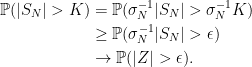
$\displaystyle \begin{aligned} {\mathbb P}(\lvert S_N\rvert > K) &= {\mathbb P}(\sigma_N^{-1}\lvert S_N\rvert > \sigma_N^{-1} K)\\ &\ge{\mathbb P}(\sigma_N^{-1}\lvert S_N\rvert > \epsilon)\\ &\rightarrow{\mathbb P}(\lvert Z\rvert > \epsilon). \end{aligned}$

Letting ${\epsilon}$ go to zero, the right hand side goes to one, giving the result.

It remains to prove the result when ${a_n}$ is an unbounded sequence, in which case we can apply a similar argument to that used in lemma 3. Then there exists a subsequence satisfying ${\lvert a_{n_k}\rvert > 2K + \lvert a_{n_{k-1}}\rvert}$ for all ${k > 1}$ . For each ${n_k\le N}$ , flipping the sign of ${X_{n_k}}$ does not impact the distribution of ${S_N}$ , but it shifts its value by ${\pm a_{n_k}}$ so, if ${\lvert S_N\rvert\le K}$ then it will be shifted to lie in the set ${A_k=[a_{n_k}-K,a_{n_k}+K]\cup[-a_{n_k}-K,-a_{n_k}+K]}$ . Hence,

$\displaystyle p_N\equiv{\mathbb P}(\lvert S_N\rvert\le K)\le{\mathbb P}(S_N\in A_k).$

The sets ${A_k}$ are disjoint so,

$\displaystyle 1\ge{\mathbb P}\left(S_N\in\bigcup\nolimits_{n_k\le N}A_k\right)=\sum_{n_k\le N}{\mathbb P}(S_N\in A_k)\ge p_N\sum_{n_k\le N}1.$

As the sum on the right tends to infinity when N goes to infinity, we have ${p_N\rightarrow0}$ . ⬜

Usually, we are concerned with the distribution of a Rademacher series ${a\cdot X}$ , rather than its particular representation as a random variable on a specific probability space. However, different values for ${a\in\ell^2}$ can lead to the same distribution. For example, flipping the signs of some elements of ${a}$ or permuting its elements has no effect on the distribution of ${a\cdot X}$ . This is because applying such operations has the same effect on ${a\cdot X}$ as applying the operations to the terms of X which, again, do not affect its distribution. Alternatively, we can see that the characteristic function (1) is unaffected by such operations.

I will use ${\ell^2_d}$ to denote the sequences ${a\in\ell^2}$ which are nonnegative and decreasing,

$\displaystyle a_1\ge a_2\ge a_3\ge\cdots\ge0.$

Any ${a\in\ell^2}$ can be put in standard form by flipping the sign of any negative terms and then arranging in decreasing order. Using ${a^*}$ for this standard form, then ${a^*\in\ell^2_d}$ and the terms ${a^*_n}$ are the same as ${\lvert a_n\rvert}$ when arranged in decreasing order. Also,

$\displaystyle a^*\cdot X\overset{d}=a\cdot X,$

where ${\overset{d}=}$ denotes equality in distribution. So, when looking at the distributions of Rademacher series, we can always assume that the weights ${a}$ are in ${\ell^2_d}$ . Once we do this, then there is no remaining degeneracy.

Lemma 9 Let X be a Rademacher series. Then, any ${a\in\ell^2_d}$ is uniquely determined by the distribution of ${a\cdot X}$ .

Proof: From expression (1) for the characteristic function ${\varphi(\lambda)={\mathbb E}[\exp(i\lambda a\cdot X)]}$ , we can express ${a_n}$ in terms of ${a_1,a_2,\ldots,a_{n-1}}$ . Factoring

$\displaystyle \varphi(\lambda)=\varphi_n(\lambda)\prod_{m=1}^{n-1}\cos(\lambda a_m)$

then ${a_n}$ is equal to ${\pi/(2\lambda)}$ with ${\lambda}$ equal to the smallest positive zero of ${\varphi_n}$ , or is equal to zero if ${\varphi_n}$ is everywhere nonzero. ⬜

Another benefit of restricting to ${\ell^2_d}$ is that we can bound the individual terms of the sequence.

Lemma 10 If ${a\in\ell^2_d}$ then

$\displaystyle a_n\le\frac1{\sqrt n}\lVert a\rVert_2.$

Proof: As ${a_m\ge a_n}$ for ${m\le n}$ , we have

$\displaystyle \lVert a\rVert_2^2=\sum_{m=1}^\infty a_m^2\ge\sum_{m=1}^n a_m^2\ge na_n^2.$

⬜

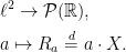
Now consider the map from a sequence ${a\in\ell^2}$ to the distribution of its Rademacher series. Using ${{\mathcal P}({\mathbb R})}$ to denote the set of Borel probability measures on ${{\mathbb R}}$ ,

$\displaystyle \begin{aligned} &\ell^2\rightarrow{\mathcal P}({\mathbb R}),\\ & a\mapsto R_a\overset{d}=a\cdot X. \end{aligned}$

We can use convergence in distribution (weak topology) on ${{\mathcal P}({\mathbb R})}$ , under which a sequence of measures ${\mu_n}$ tends to a limit ${\mu}$ iff ${\mu_n(f)\rightarrow\mu(f)}$ for all continuous bounded functions ${f\colon{\mathbb R}\rightarrow{\mathbb R}}$ . Restricting the domain to ${\ell^2_d}$ , lemma 9 says that ${a\mapsto R_a}$ is one-to-one. By corollary 2, it is also continuous with respect to the norm topology on ${\ell^2}$ and the weak topology on ${{\mathcal P}({\mathbb R})}$ . However, the norm topology is too strong for many purposes. For example, in the context of lemma 6, the sequence ${a^n}$ is not norm convergent when ${\sigma > 0}$ , but does converge weakly to zero. I will finish this post by considering how we can extend the idea of Rademacher series to naturally incorporate limits such as that given by lemma 6 into the domain of the map.

The weak topology on ${\ell^2}$ , by definition, is the weakest topology making the maps ${a\mapsto\langle a,b\rangle}$ continuous for each fixed ${b\in\ell^2}$ . In particular, a sequence ${a^n\in\ell^2}$ converges weakly to the limit ${a}$ if and only if ${\langle a^n,b\rangle\rightarrow\langle a,b\rangle}$ for each ${b\in\ell^2}$ . On any bounded set, it can be seen that weak convergence is equivalent to the pointwise convergence of the terms in the sequences (or, the product topology).

Looking again at lemma 6, we see that the sequence ${a^n}$ is weakly convergent, but that ${a^n\cdot X}$ convergences in distribution to a Gaussian. This suggests completing the space of Rademacher series distributions by adding in a Gaussian term. I do this as follows. First, let ${({\mathbb R}\oplus\ell^2)_d}$ consist of the pairs ${(\sigma,a)}$ for ${\sigma\in{\mathbb R}}$ and ${a\in\ell^2_d}$ with ${\sigma\ge\lVert a\rVert_2}$ . Weak convergence in this space is the same as weak convergence separately for ${a}$ and ${\sigma}$ , which the same as pointwise convergence of ${\sigma}$ and the terms of ${a}$ . Next, let X be a Rademacher sequence and Y be an independent normal random variable with zero mean and unit variance. Then, define the map

$\displaystyle \begin{aligned} &({\mathbb R}\oplus\ell^2)_d\rightarrow{\mathcal P}({\mathbb R}),\\ &(\sigma,a)\mapsto R_{\sigma,a} \overset{d}= S_{\sigma,a}\equiv a\cdot X + (\sigma^2-\lVert a\rVert_2^2)^{1/2}Y. \end{aligned}$

(3)

In the case that ${\sigma=\lVert a\rVert_2}$ , this is just the distribution of the Rademacher series ${a\cdot X}$ . However, we are allowing an additional normal term by taking ${\sigma > \lVert a\rVert_2}$ , and it is straightforward to see that ${R_{\sigma,a}}$ has variance ${\sigma^2}$ .

Lemma 11 The map ${(\sigma,a)\mapsto R_{\sigma,a}}$ is weakly continuous and one-to-one, and is a weak homeomorphism onto its image.

Proof: Using (1), we can compute the characteristic function,

$\displaystyle \varphi_{\sigma,a}(\lambda)\equiv{\mathbb E}[e^{i\lambda S_{\sigma,a}}]=e^{-\frac{\lambda^2}2\sigma^2}\prod_{n=1}^\infty e^{\frac{\lambda^2}2a_n^2}\cos(\lambda a_n).$

To see that this is one-to-one, we need to show that ${(\sigma,a)}$ can be recovered from knowledge of the characteristic function. This is straightforward: ${\sigma^2}$ is equal to the variance, and ${a}$ can be recovered in exactly the same way as in the proof of lemma 9.

We next show continuity. So, suppose that ${(\sigma_n,a^n)}$ converges weakly to ${(\sigma,a)}$ . We need to show that ${\varphi_{\sigma_n,a^n}(\lambda)\rightarrow\varphi_{\sigma,a}(\lambda)}$ for each fixed ${\lambda}$ . First, as it converges, ${\sigma_n}$ is bounded above by some ${K\in{\mathbb R}}$ . Then, ${a^n_m\le K/\sqrt{m}}$ so, fixing positive ${\epsilon < \pi/2}$ , for sufficiently large ${N}$ we have ${\lvert \lambda a^n_N\rvert\le\epsilon}$ . As ${\cos(\lambda a^n_m)}$ is nonnegative over ${m\ge N}$ , we can express the characteristic function as

$\displaystyle \varphi_{\sigma_n,a^n}(\lambda) =e^{-\frac{\lambda^2}2\sigma^2_n} \exp\left(\sum_{m=N}^\infty(\frac12(\lambda a^n_m)^2+\log\cos(\lambda a^n_m))\right)\prod_{m=1}^{N-1} e^{\frac12(\lambda a^n_m)^2}\cos(\lambda a^n_m).$

The terms on the right hand side manifestly converge as ${n\rightarrow\infty}$ , except for the term in the exponential where we need to commute the limit with the infinite sum. As ${x^2/2+\log\cos(x)}$ is of order ${x^4}$ , it is bounded by ${Lx^4}$ for some positive ${L}$ . So, the terms inside the sum on the right hand side are bounded by ${L\lambda^4(a^n_m)^4\le K^4L\lambda^4/m^2}$ , which has finite sum over ${m}$ . Hence, by dominated convergence, we can commute the limit with the infinite sum and we obtain

$\displaystyle \varphi_{\sigma_n,a^n}(\lambda)\rightarrow\varphi_{\sigma,a}(\lambda)$

as required.

It just remains to show that the inverse of ${(\sigma,a)\mapsto R_{\sigma,a}}$ is weakly continuous. For each fixed ${K > 0}$ , the space of ${(\sigma,a)\in({\mathbb R}\oplus\ell^2)_d}$ with ${\sigma\le K}$ is compact (by Tychonoff’s theorem) so, restricting to such bounded sets, the result is immediate. Every continuous one-to-one map from a compact space to a Hausdorff space has continuous inverse. Hence, we just need to show that if ${(\sigma_n,a^n)\in({\mathbb R}\oplus\ell^2)_d}$ is a sequence such that ${R_{\sigma_n,a^n}\rightarrow R_{\sigma,a}}$ weakly, then ${\sigma_n}$ is a bounded sequence. I will use the fact that if ${\lambda_n\in{\mathbb R}}$ is a sequence tending to zero then ${\varphi_{\sigma_n,a^n}(\lambda_n)\rightarrow1}$ .

First, we can show that ${a^n_1}$ is a bounded sequence. If not then, by passing to a subsequence, we can suppose that ${a^n_1\rightarrow\infty}$ . Setting ${\lambda_n=\pi/(2a_1^n)\rightarrow0}$ gives ${\varphi_{\sigma_n,a^n}(\lambda_n)=0}$ , a contradiction. Next, we show that ${\sigma_n}$ is bounded. If not then, by passing to a subsequence, we can suppose that ${\sigma_n\rightarrow\infty}$ . Taking ${\lambda_n=\sigma_n^{-1}\rightarrow0}$ then ${\lambda_n a^n_1 < \pi/2}$ for large n, so we obtain the contradiction

$\displaystyle \varphi_{\sigma_n,a^n}(\lambda_n)\le e^{-\frac12\lambda_n^2\sigma_n^2}=e^{-\frac12} < 1.$

⬜

In fact, for any ${(\sigma,a)\in({\mathbb R}\oplus\ell^2)_d}$ , it is not difficult to construct a sequence ${a^n\in\ell^2_d}$ converging weakly to ${a}$ such that ${\lVert a^n\rVert_2=\sigma}$ . Then, ${(\sigma,a^n)}$ tends weakly to ${(\sigma,a)}$ and, by the above result,

$\displaystyle a^n\cdot X\overset{d}\rightarrow R_{\sigma,a}.$

Hence, the definition above given for ${R_{\sigma,a}}$ is the unique continuous extension of the Rademacher series distribution to all of ${({\mathbb R}\oplus\ell^2)_d}$ . Furthermore, we see that the set of measures

$\displaystyle \left\{R_{\sigma,a}\colon(\sigma,a)\in({\mathbb R}\oplus\ell^2)_d\right\}$

is the weak closure of the distributions of Rademacher series, and is weakly homeomorphic to ${({\mathbb R}\oplus\ell^2)_d}$ .

One benefit of using the map (3) together with the weak topology is that the unit ball of ${\ell^2}$ (and, hence, of ${\ell^2_d}$ ) is weakly compact. Using ${(\ell^2_d)_1}$ to denote the unit ball, we obtain a continuous map

$\displaystyle \begin{aligned} & (\ell^2_d)_1\rightarrow{\mathcal P}({\mathbb R}),\\ & a\mapsto R_{1,a}. \end{aligned}$

This is equal to the distribution of ${a\cdot X}$ when ${\lVert a\rVert_2=1}$ , and is a weak homeomorphism onto its image.

	Anonymous on About
	Anonymous on About
	Anonymous on The Stochastic Integral
	Anonymous on Bessel Processes
	Anonymous on Bessel Processes
	Stat Prof on Pathwise Regularity of Optiona…
	Yang Chu on Spitzer’s Formula
	Anonymous on About
	Anonymous on Continuous Processes with Inde…
	Anonymous on Continuous Processes with Inde…

Rademacher Series

Published by George Lowther

One thought on “Rademacher Series”

Leave a comment Cancel reply

Related

Published by George Lowther

One thought on “Rademacher Series”

Leave a comment Cancel reply