The Khintchine Inequality

For a Rademacher sequence ${X=(X_1,X_2,\ldots)}$ and square summable sequence of real numbers ${a=(a_1,a_2,\ldots)}$ , the Khintchine inequality provides upper and lower bounds for the moments of the random variable,

$\displaystyle a\cdot X=a_1X_1+a_2X_2+\cdots.$

We use ${\ell^2}$ for the space of square summable real sequences and

$\displaystyle \lVert a\rVert_2=\left(a_1^2+a_2^2+\cdots\right)^{1/2}$

for the associated Banach norm.

Theorem 1 (Khintchine) For each ${0 < p < \infty}$ , there exists positive constants ${c_p,C_p}$ such that,

$\displaystyle c_p\lVert a\rVert_2^p\le{\mathbb E}\left[\lvert a\cdot X\rvert^p\right]\le C_p\lVert a\rVert_2^p,$ (1)

for all ${a\in\ell^2}$ .

Note the similarity to the Burkholder-Davis-Gundy inequality. In fact, the process ${S_N=\sum_{n=1}^Na_nX_n}$ is a martingale, with time index N. Then, the quadratic variation ${[S]_\infty}$ is equal to ${\lVert a\rVert_2^2}$ , and (1) can be regarded as a special case of the BDG inequality — at least, when p is greater than one. However, the Khintchine inequality is much easier to prove. I will give a proof in a moment but, first, there are some simple observations that can be made. We already know, from the previous post, that the map ${a\mapsto a\cdot X}$ is an isometry between ${\ell^2}$ and ${L^2}$ . That is,

$\displaystyle {\mathbb E}[(a\cdot X)^2]=\lVert a\rVert_2^2.$

So, the Khintchine inequality for ${p=2}$ is trivial, and we can take ${c_2=C_2=1}$ . Also, it is a simple application of Jensen’s inequality to show that ${{\mathbb E}[Z^p]^{1/p}}$ is increasing in p, for any nonnegative random variable Z. Specifically, for ${p < q}$ , convexity of the map ${x\mapsto x^{q/p}}$ gives,

$\displaystyle {\mathbb E}[Z^p]^{1/p}=\left({\mathbb E}[Z^p]^{q/p}\right)^{1/q}\le{\mathbb E}[Z^q]^{1/q}.$

Hence,

$\displaystyle {\mathbb E}[\lvert a\cdot X\rvert^p]\le{\mathbb E}[(a\cdot X)^2]^{p/2}=\lVert a\rVert_2^p$

for all ${p\le 2}$ . We immediately see that the right-hand Khintchine inequality holds with ${C_p=1}$ for ${p\le 2}$ . Similarly, for ${p\ge2}$ ,

$\displaystyle {\mathbb E}[\lvert a\cdot X\rvert^p]\ge{\mathbb E}[(a\cdot X)^2]^{p/2}=\lVert a\rVert_2^p,$

and we see that the left-hand Khintchine inequality holds with ${c_p=1}$ . So, the only non-trivial cases of (1) are the left-hand inequality for ${p < 2}$ and the right-hand one for ${p > 2}$ .

Proof of Theorem 1: We start with the right-hand inequality, by making use of inequality (2) from the previous post,

$\displaystyle \begin{aligned} {\mathbb E}[\cosh(\lambda a\cdot X)] &=\frac12{\mathbb E}[e^{\lambda a\cdot X}+e^{-\lambda a\cdot X}]\\ &\le e^{\frac12\lambda^2\lVert a\rVert_2^2}, \end{aligned}$

for any fixed positive ${\lambda}$ . Since ${\cosh(x)}$ grows faster than ${x^p}$ , for any ${0 < p < \infty}$ , there exists a positive constant ${B_p}$ satisfying ${\lvert x\rvert^p\le B_p\cosh(x)}$ . Hence,

$\displaystyle \lambda^p{\mathbb E}[\lvert a\cdot X\rvert^p]\le B_p{\mathbb E}[\cosh(\lambda a\cdot X)]\le B_p e^{\frac12\lambda^2\lVert a\rVert_2^2}.$

Dividing ${\lambda}$ by ${\lVert a\rVert_2}$ gives

$\displaystyle {\mathbb E}[\lvert a\cdot X\rvert^p]\le C_p\lVert a\rVert_2^p.$

with the constant ${C_p=\lambda^{-p}B_p\exp(\lambda^2/2)}$ .

The left-hand Khintchine inequality follows from the right-hand one, by making use of the fact that ${{\mathbb E}[\lvert a\cdot X\rvert^p]}$ is log-convex in p (see lemma 2 below). Since we have already noted that ${c_p=1}$ for ${p\ge2}$ , we assume that ${p < 2}$ . Choosing any ${q > 2}$ , log-convexity gives

$\displaystyle \begin{aligned} \lVert a\rVert_2^{2(q-p)} &={\mathbb E}[\lvert a\cdot X\rvert^2]^{q-p}\\ &\le{\mathbb E}[\lvert a\cdot X\rvert^p]^{q-2}{\mathbb E}[\lvert a\cdot X\rvert^q]^{2-p}\\ &\le{\mathbb E}[\lvert a\cdot X\rvert^p]^{q-2}C_q^{2-p}\lVert a\rVert_2^{q(2-p)}. \end{aligned}$

Rearranging gives the result with ${c_p=C_q^{(p-2)/(q-2)}}$ . ⬜

A function ${f\colon(0,\infty)\rightarrow{\mathbb R}^+\cup\{\infty\}}$ is log-convex if ${\log f(x)}$ is convex or, equivalently,

$\displaystyle f(r)\le f(p)^{\frac{q-r}{q-p}}f(q)^{\frac{r-p}{q-p}}$

for all ${p < r < q}$ . In the proof above, I made use of log-convexity of the moments. This is equivalent to the statement that moment generating functions are log-convex. For completeness, I include a brief proof of this standard fact.

Lemma 2 Let Z be a nonnegative random variable. Then, ${{\mathbb E}[Z^p]}$ is log-convex over ${0 < p < \infty}$ .

Proof: One method is to simply differentiate ${\log{\mathbb E}[Z^p]}$ twice with respect to p. Alternatively, for ${p < r < q}$ , set ${p^\prime=(q-p)/(q-r)}$ and ${q^\prime=(q-p)/(r-p)}$ so that ${1/p^\prime+1/q^\prime=1}$ . Applying Hölder’s inequality gives the result,

$\displaystyle {\mathbb E}[Z^r] ={\mathbb E}\left[Z^{\frac{p}{p^\prime}}Z^{\frac{q}{q^\prime}}\right] \le{\mathbb E}[Z^p]^{\frac1{p^\prime}}{\mathbb E}[Z^q]^{\frac1{q^\prime}}.$

⬜

An alternative way of looking at the Khintchine inequality is that it says that, on the space of Rademacher series, the ${L^p}$ topologies all coincide. I will use ${\lVert X\rVert_p}$ to denote ${{\mathbb E}[\lvert Z\rvert^p]^{1/p}}$ . Over ${p\ge1}$ , it is well-known that this is a Banach norm. However, it defines a topology for each ${0 < p < \infty}$ , so that convergence of a sequence of random variables ${Z_n}$ to a limit ${Z}$ in the ${L^p}$ topology is equivalent to ${\lVert Z_n-Z\rVert_p\rightarrow0}$ .

Lemma 3 Let V be a linear subspace of ${L^p\cap L^q}$ for some ${0 < p,q < \infty}$ . v Then, the ${L^p}$ and ${L^q}$ topologies are equivalent on V if and only if there exists positive constants ${c,C}$ satisfying,

$\displaystyle c\lVert Z\rVert_q\le\lVert Z\rVert_p\le C\lVert Z\rVert_q$ (2)

for all ${Z\in V}$ .

Proof: First, if (2) holds, then it is immediate that a sequence converges in ${L^p}$ if and only if it converges in ${L^q}$ , so we look at the converse. Using proof by contradiction, suppose that there was no constant C for which the right-hand inequality holds. Then, there exists a sequence ${Z_n\in V}$ such that ${\lVert Z_n\rVert_p > n\lVert Z_n\rVert_q}$ . By scaling, we can assume that ${\lVert Z_n\rVert_p=1}$ . However, this gives ${\lVert Z_n\rVert_q\le1/n\rightarrow0}$ so, by assumption, we also have convergence in the ${L^p}$ topology giving the contradiction ${1=\lVert Z_n\rVert_p\rightarrow0}$ .

We have shown that the right-hand inequality of (2) holds for some positive constant C, and the left hand inequality follows by exchanging the role of p and q. ⬜

These ideas extend to the ${L^0}$ topology, which is just convergence in probability.

Lemma 4 Let V be a linear subspace of ${L^p}$ for some ${0 < p < \infty}$ . Then, the ${L^0}$ and ${L^p}$ topologies are equivalent on V if and only if there exists strictly positive constants ${\epsilon,\delta}$ satisfying,

$\displaystyle {\mathbb P}(\lvert Z\rvert\ge\epsilon\lVert Z\rVert_p)\ge\delta$ (3)

for all ${Z\in V}$ .

Proof: First, it is standard that convergence in in the ${L^p}$ topology implies convergence in probability. To be explicit, if ${\lVert Z_n\rVert_p\rightarrow0}$ for a sequence ${Z_n\in V}$ then, for each ${\epsilon > 0}$ ,

$\displaystyle \begin{aligned} {\mathbb P}(\lvert Z_n\rvert \ge \epsilon) &={\mathbb E}[1_{\{\lvert Z_n\rvert\ge\epsilon\}}]\le{\mathbb E}[\epsilon^{-p}\lvert Z_n\rvert^p]\\ &=\epsilon^{-p}\lVert Z_n\rVert_p^p\rightarrow0 \end{aligned}$

as required. Conversely, suppose that (3) holds for given ${\epsilon_\delta}$ and that ${Z_n}$ tends to zero in probability. We need to show that ${\lVert Z_n\rVert_p\rightarrow0}$ . If this was not the case then, by passing to a subsequence, we would have ${\lVert Z_n\rVert_p\ge K}$ for some fixed positive K. So,

$\displaystyle {\mathbb P}(\lVert Z_n\rVert\ge\epsilon\lVert Z_n\rVert_p) \le{\mathbb P}(\lVert Z_n\rVert\ge\epsilon K)\rightarrow0,$

contradicting (3).

Finally, supposing that the ${L^p}$ and ${L^0}$ topologies coincide, we just need to show that (3) holds. I use proof by contradiction so, suppose that (3) does not hold for any ${\epsilon,\delta > 0}$ . Then, there exists a sequence ${Z_n\in V}$ satisfying

$\displaystyle {\mathbb P}(\lvert Z_n\rvert\ge\lVert Z_n\rVert_p/n) < 1/n.$

By scaling, we can suppose that ${\lVert Z_n\rVert_p=1}$ so that, in particular, the sequence does not tend to zero in ${L^p}$ . However, for any ${alpha > 0}$ we have

$\displaystyle {\mathbb P}(\lvert Z_n\rvert\ge\alpha) < 1/n\rightarrow0$

for ${n\ge\alpha^{-1}}$ . This shows that ${Z_n}$ tends to zero in ${L^0}$ but not in ${L^p}$ , contradicting the initial assumption. ⬜

Statements such as (3) are known as anti-concentration inequalities, and bound, from above, the probability that a random variable can be within a given distance of its mean. So, to show the equivalence of the ${L^0}$ and ${L^p}$ topologies for Rademacher series, it is only really necessary to prove a single non-trivial anti-concentration inequality.

Lemma 5 Let X be a Rademacher sequence and ${a\in\ell^2}$ . Then,

$\displaystyle {\mathbb P}(\lvert a\cdot X\rvert\ge x\lVert a\rVert_2)\ge\frac13(1-x^2)^2$ (4)

for all ${0 < x < 1}$ .

Proof: Using ${Z=\lvert a\cdot X\rvert}$ , the Paley-Zygmund inequality gives

$\displaystyle \begin{aligned} {\mathbb P}(Z \ge x\lVert a\rVert_2) &={\mathbb P}(Z^2\ge x^2{\mathbb E}[Z^2])\\ &\ge(1-x^2)^2\frac{{\mathbb E}[Z^2]^2}{{\mathbb E}[Z^4]}\\ &\ge\frac1{C_4}(1-x^2)^2. \end{aligned}$

Here, the left-hand Khintchine inequality was used in the final inequality. In fact, we can use ${C_4=3}$ , giving (4).

Note that ${X_{n_1}X_{n_2}\cdots X_{n_r}}$ is antisymmetric in flipping the sign of ${X_{n_1}}$ whenever ${n_1\not\in\{n_2,\ldots,n_r\}}$ , so has zero expectation. Hence, writing ${S_N=\sum_{n=1}^Na_nX_n}$ , we obtain

$\displaystyle \begin{aligned} {\mathbb E}[S_N^4] &=\sum_{n=1}^Na_n^4+6\sum_{1\le m < n\le N}a_ma_n\\ &=3\left(\sum_{n=1}^Na_n^2\right)^2-2\sum_{n=1}^Na_n^4. \end{aligned}$

Letting N go to infinity, and using convergence in ${L^4}$ ,

$\displaystyle {\mathbb E}[\lvert a\cdot X\rvert^4]=3\lVert a\rVert_2^4-2\sum_{n=1}^\infty a_n^4\le3\lVert a\rVert_2^4.$

So, ${C_4=3}$ as claimed. ⬜

Combining with lemma 4, this result shows that the ${L^2}$ and ${L^0}$ topologies coincide for Rademacher series. Similarly, lemma 3 shows that the Khintchine inequality is equivalent to stating that the ${L^p}$ topologies coincide for all ${0 < p < \infty}$ . Hence, we obtain the following alternative statement of the Khintchine inequalities, which naturally incorporates the ${L^0}$ version.

Theorem 6 The space ${\{a\cdot X\colon a\in\ell^2\}}$ is contained in ${L^p}$ for all ${0\le p < \infty}$ and, for all ${0\le p,q < \infty}$ , the ${L^p}$ and ${L^q}$ topologies are equivalent on this space.

Although this statement unites the Khintchine inequalities for ${p > 0}$ with the corresponding version for ${p=0}$ , when expressed as explicit quantitative statements as in (1) and (4), they do look rather different. For ${p > 0}$ , the inequality is of the form

$\displaystyle g(\lVert a\rVert_2)\le{\mathbb E}[F(\lvert a\cdot X\rvert)]\le G(\lVert a\rVert_2)$

for some increasing functions ${F,G,g\colon{\mathbb R}_+\rightarrow{\mathbb R}_+}$ . The left-hand inequality for the ${p=0}$ case can also be expressed in a similar style.

Lemma 7 For a random variable Z, inequality (3) holds if and only if

$\displaystyle {\mathbb E}[F(\lvert Z\rvert)]\ge\delta F(\epsilon\lVert Z\rVert_p)$ (5)

for all increasing functions ${F\colon{\mathbb R}_+\rightarrow{\mathbb R}_+}$ .

Proof: If (5) holds, then (3) follows immediately by taking ${F(x)=1_{\{x\ge\epsilon\lVert Z\rVert_p\}}}$ . Conversely, if (3) holds then,

$\displaystyle \begin{aligned} E[F(\lvert Z\rvert)] &\ge{\mathbb E}\left[1_{\{Z\ge\epsilon\lVert Z\rVert_p\}}F(\epsilon\lVert Z\rVert_p)\right]\\ &={\mathbb P}(\lvert Z\rvert\ge\epsilon\lVert Z\rVert_p)F(\epsilon\lVert Z\rVert_p)\\ &\ge\delta F(\epsilon\lVert Z\rVert_p), \end{aligned}$

as required. ⬜

The (left-hand) ${L^0}$ Khintchine inequality is then expressed by

$\displaystyle \delta F(\epsilon\lVert a\rVert_2)\le{\mathbb E}[F(\lvert a\cdot X\rvert)].$

for some constants ${\epsilon,\delta > 0}$ and every increasing function ${F\colon{\mathbb R}_+\rightarrow{\mathbb R}_+}$ . This form also makes clear that the ${L^p}$ left-hand inequality for all ${p > 0}$ follows from the ${L^0}$ version. We simply take ${F(x)=x^p}$ and ${c_p=\delta\epsilon^p}$ .

Although the Khintchine inequality is only concerning Rademacher sequences, it does have implications for much more general sequences. For example, the following consequence does not place any restriction on the distribution of the random variables ${Z_n}$ , which are not even required to be independent. This was central to the construction of the stochastic integral given earlier in my notes, which only required the most basic properties of semimartingales.

Theorem 8 Let ${Z_1,Z_2,\ldots}$ be a sequence of random variables in ${L^p}$ such that the set

$\displaystyle S=\left\{\sum_{k=1}^n Z_kr_k\colon n\in{\mathbb N},r_1,\ldots,r_n\in\{\pm1\}\right\}$ (6)

is ${L^p}$ bounded, for some ${0\le p < \infty}$ . Then, ${\left(\sum_{n=1}^\infty Z_n^2\right)^{1/2}}$ is in ${L^p}$ .

Proof: Set ${\sigma_n=(\sum_{k=1}^nZ_k^2)^{1/2}}$ . Then, if ${\mu}$ is the uniform probability measure on ${\{\pm1\}^n}$ , we can write

$\displaystyle F(\sigma_n)\le\int G\left(\sum\nolimits_{k=1}^nZ_kr_k\right)d\mu(r).$

for some ${F(x),G(x)}$ which are increasing unbounded functions of ${\lvert x\rvert}$ . Specifically for ${p > 0}$ , the left-hand Khintchine inequality says that this holds with ${F(x)=\lvert x\rvert^p}$ and ${G(x)=c_p^{-1}\lvert x\rvert^p}$ . For ${p=0}$ , lemma 7 says that we can choose ${G}$ however we like, and ${F(x)}$ of the form ${\delta^{-1}G(\epsilon^{-1}x)}$ . We choose ${G}$ to be left-continuous and, by boundedness in probability, such that ${{\mathbb E}[G(Z)]}$ is bounded over ${Z\in S}$ .

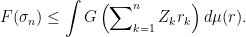
In either case, we can take expectations,

$\displaystyle {\mathbb E}[F(\sigma_n)]\le\int{\mathbb E}\left[G\left(\sum\nolimits_{k=1}^nZ_kr_k\right)\right]d\mu(r),$

and the right hand side is bounded by some constant K independently of n. Hence, letting n go to infinity and applying Fatou’s lemma on the left gives

$\displaystyle {\mathbb E}\left[F\left(\left(\sum\nolimits_{k=1}^\infty Z_k^2\right)^{1/2}\right)\right] \le K < \infty$

as required. ⬜

The conclusion of theorem 8 directly implies that the sequence converges to zero in the ${L^p}$ topology. It was this consequence which was important in my construction of the stochastic integral.

Corollary 9 Let ${Z_1,Z_2,\ldots}$ be a sequence of random variables such that the set (6) is ${L^p}$ bounded, for some ${0\le p < \infty}$ . Then, ${Z_n\rightarrow0}$ in ${L^p}$ .

Proof: Since theorem 8 says that ${\sigma_\infty\equiv(\sum_{n=1}^\infty Z_n^2)^{1/2}}$ is in ${L^p}$ and, in particular, is almost surely finite, we see that ${Z_n\rightarrow0}$ almost surely. This implies that ${Z_n\rightarrow0}$ in ${L^0}$ and, for ${p > 0}$ , as ${\lvert Z_n\rvert\le\sigma_\infty}$ , dominated convergence gives ${Z_n\rightarrow0}$ in ${L^p}$ . ⬜

I only made use of the ${L^0}$ version of corollary 9 in the construction of the stochastic integral, as this is sufficient for the property of bounded convergence in probability. However, the corollary can also be used in its ${p > 0}$ versions to obtain an ${L^p}$ theory of stochastic integration. For a semimartingale X, we require that

$\displaystyle \left\{\int_0^t\xi\,dX\colon\lvert\xi\rvert\le1{\rm\ is\ elementary}\right\}$

is ${L^p}$ bounded, for each positive time t. The resulting stochastic integral will then satisfy bounded convergence in ${L^p}$ . This approach dates back to the 1981 paper Stochastic Integration and L^p-Theory of Semimartingales by Bichteler, and is used in his book Stochastic Integration with Jumps.

Note that the statement of corollary 9 makes sense in any topological vector space. So, for any such space V, we can ask whether, for every sequence ${z_n\in V}$ such that the set

$\displaystyle \left\{\sum_{k=1}^n r_kz_k\colon n\in{\mathbb N},r_1,\ldots,r_n\in\{\pm1\}\right\}$

is bounded, does ${z_n}$ necessarily tend to zero? It is not difficult to show that this is true in Hilbert spaces and, more generally, in uniformly convex spaces. However, it does not hold in all spaces. Take, for example, ${V=\ell^\infty}$ , which is the space of bounded real sequences ${(a_1,a_2,\ldots)}$ under uniform convergence. Then consider ${z_n\in\ell^\infty}$ such that ${(z_n)_m=0}$ for ${m\not=n}$ and ${(z_n)_n=1}$ . The sums ${\sum_{k=1}^nr_kz_k}$ all have uniform norm equal to 1, so form a bounded set. However, ${z_n}$ does not tend to zero.

The ${L^p}$ spaces for ${p\le1}$ fail many of the usual `nice’ properties that are often required when working with topological vector spaces. For example, ${L^1}$ is generally not uniformly convex and, for ${p < 1}$ , ${L^p}$ is not even locally convex. So, corollary 9 gives a fundamental and nontrivial property that ${L^p}$ spaces do satisfy, and which is sufficient to ensure a well behaved theory of stochastic integration.

Optimal Khintchine Constants

In the discussion above, I paid no concern to the optimal values of the constants in the Khintchine inequality. All that we were concerned with is that finite and positive constants do exist. However, the inequality is clearly improved if ${C_p}$ can be made as small as possible, and ${c_p}$ is as large as possible. In fact, the optimal values of these constants are known. I will not give full proofs here, but the actual values are enlightening, so I will mention them, and prove the `easy’ case of ${C_p}$ over ${p\ge3}$ .

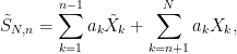
Use ${\gamma_p}$ to denote the p‘th absolute Gaussian moment, which can be computed explicitly in terms of the gamma function. Letting N be a standard normal random variable, on some probability space,

$\displaystyle \begin{aligned} \gamma_p &\equiv{\mathbb E}[\lvert N\rvert^p]\\ &=2^{\frac p2}\pi^{-\frac12}\Gamma\left(\frac{p+1}2\right). \end{aligned}$

It is straightforward (using Jensen’s inequality) to show that ${\gamma_p}$ is strictly increasing in p, and ${\gamma_2=1}$ . So, ${\gamma_p > 1}$ for ${p > 2}$ and ${\gamma_p < 1}$ for ${p < 2}$ . It turns out that, over ${p\ge2}$ , moments of Khintchine series are bounded above by Gaussian moments.

Theorem 10 The optimal Khintchine constants are,

$\displaystyle \begin{aligned} &C_p=\max(1,\gamma_p),\\ &c_p=\min(1,\gamma_p,2^{p/2-1}). \end{aligned}$ (7)

The first thing to note is that, for any p, it is always possible to achieve the bounds given in (7) or, at least, approximate them as closely as we like. Specifically, consider ${a\in\ell^2}$ with ${\lVert a\rVert_2=1}$ in the following cases.

If ${a_1=1}$ then ${{\mathbb E}[\lvert a\cdot X\rvert^p]=1}$ .
If ${a_1=a_2=1/\sqrt2}$ then ${{\mathbb E}[\lvert a\cdot X\rvert^p]=2^{p/2-1}}$ .
By lemma 6 of the post on Rademacher series, if we let ${\lVert a\rVert_\infty}$ go to zero then ${{\mathbb E}[\lvert a\cdot X\rvert^p]\rightarrow\gamma_p}$ .

This shows that, if it can be shown that the Khintchine inequality holds with the constants in (7), then it is optimal. We already noted above that the inequality holds with ${C_p=1}$ for ${p\le2}$ and ${c_p=1}$ for ${p\ge2}$ , so this is optimal. The remaining cases are,

$\displaystyle \begin{aligned} &C_p=\gamma_p,{\rm\ for\ }p > 2,\\ &c_p=\min(\gamma_p,2^{p/2-1}),{\rm\ for\ }p < 2. \end{aligned}$

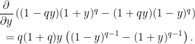
Incidentally, we already showed that ${C_4=\gamma_4=3}$ in the process of proving lemma 5. A similar method, simply expanding out the power of the series, can be applied for all even integer p.

Lemma 11 For each even integer ${p\ge2}$ , the Khintchine inequality holds with ${C_p=\gamma_p}$ .

Proof: Writing ${S_N=\sum_{n=1}^Na_nX_n}$ , expanding the power of the sum gives

$\displaystyle S_N^p=\sum_{i_1,\ldots,i_p=1}^Na_{i_1}\cdots a_{i_p}X_{i_1}\cdots X_{i_p}.$

(8)

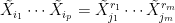
For the product of the X‘s, by collecting together equal terms, we can write

$\displaystyle X_{i_1}\cdots X_{i_p}=X_{j_1}^{r_1}\cdots X_{j_m}^{r_m}$

where the ${j_k}$ are distinct. By symmetry in switching the sign of ${X_j}$ , if any of the powers ${r_k}$ are odd, then this will have zero expectation. On the other hand, if all of the powers are even, then it is equal to 1.

In order to simplify relating this sum to ${\gamma_p}$ , we employ a devious trick. Let ${\tilde X_1,\tilde X_2,\ldots}$ be an IID sequence of standard normal random variables defined on some probability space. As above,

$\displaystyle \tilde X_{i_1}\cdots \tilde X_{i_p}=\tilde X_{j_1}^{r_1}\cdots \tilde X_{j_m}^{r_m}$

will have zero mean if any of the powers ${r_k}$ are odd and, if they are all even then,

$\displaystyle \begin{aligned} {\mathbb E}[\tilde X_{i_1}\cdots \tilde X_{i_p}] &={\mathbb E}[\tilde X_{j_1}^{r_1}]\cdots{\mathbb E}[\tilde X_{j_m}^{r_m}]\\ &=\gamma_{r_1}\cdots\gamma_{r_m}\ge1. \end{aligned}$

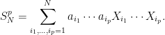
In any case, if we set 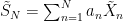${\tilde S_N=\sum_{n=1}^Na_n\tilde X_n}$ then taking expectations of (8) gives,

$\displaystyle \begin{aligned} {\mathbb E}[S_N^p] &=\sum_{i_1,\ldots,i_p=1}^Na_{i_1}\cdots a_{i_p}{\mathbb E}[X_{i_1}\cdots X_{i_p}]\\ &\le\sum_{i_1,\ldots,i_p=1}^Na_{i_1}\cdots a_{i_p}{\mathbb E}[\tilde X_{i_1}\cdots\tilde X_{i_p}]\\ &={\mathbb E}[\tilde S_N^p]. \end{aligned}$

As sums of independent normals are normal, ${\tilde S_N}$ is normal with variance ${\sigma_N^2=\sum_{n=1}^Na_n^2}$ ,

$\displaystyle {\mathbb E}[S_N^p]\le{\mathbb E}[\tilde S_N^p]=\gamma_p\sigma_N^p\le\gamma_p\lVert a\rVert_2^p$

Finally, letting N go to infinity and applying Fatou’s lemma on the left hand side gives the result. ⬜

I extend this result to all real ${p\ge3}$ . As we can no longer simply expand out the power of the sum, a convexity argument employing Jensen’s inequality will be used.

Lemma 12 For each ${p\ge3}$ , the function

$\displaystyle f(x)=(1+\sqrt x)^p+\lvert1-\sqrt x\rvert^p$

is convex on the nonnegative reals.

Proof: Differentiating ${f}$ twice, and using ${q=1/(p-2)}$ and ${y=\sqrt x/q}$ , gives

$\displaystyle \frac{4x^{3/2}}{p}f^{\prime\prime}(x)=\lvert1-qy\rvert^{\frac1q}(y+1)+(1+qy)^{\frac1q}(y-1).$

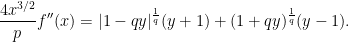
Note that both terms on the right are positive so long as ${y\ge1}$ . On the other hand, for ${y\le1}$ , compute the derivative

$\displaystyle \begin{aligned} &\frac{\partial}{\partial y}\left((1-qy)(1+y)^q-(1+qy)(1-y)^q\right)\\ &\ =q(1+q)y\left((1-y)^{q-1}-(1+y)^{q-1}\right). \end{aligned}$

As ${q\le1}$ , this is nonnegative, so

$\displaystyle (1-qy)(1+y)^q\ge(1+qy)(1-y)^q$

and substituting into the expression for ${f^{\prime\prime}}$ gives ${f^{\prime\prime}\ge0}$ as required. ⬜

Unfortunately, for ${2 < p < 3}$ , the function in lemma 12 is not convex, and a different approach is required. I concentrate on ${p\ge3}$ . We will use a similar trick as in lemma 11 whereby we replace the Rademacher random variables by normals. To simplify the argument a bit, rather than replacing them all in one go, here we will replace them one at a time.

Lemma 13 For each real ${p\ge3}$ , the Khintchine inequality holds with ${C_p=\gamma_p}$ .

Proof: Applying lemma 12, and scaling, the function

$\displaystyle f(x)=\frac12\left(\lvert a+b\sqrt x\rvert^p+\lvert a-b\sqrt x\rvert^p\right)$

is convex for any real ${a,b}$ . Hence, if X is a Rademacher random variable and Y is standard normal, then ${{\mathbb E}[Y^2]=1}$ and Jensen’s inequality gives

$\displaystyle {\mathbb E}[\lvert a+bX\rvert^p]=f(1) \le{\mathbb E}[f(Y^2)] ={\mathbb E}[\lvert a+bY\rvert^p].$

Next, if S is any random variable and X, Y are as above, independently of S, then

$\displaystyle \begin{aligned} {\mathbb E}[\lvert S+bX\rvert^p] &={\mathbb E}[{\mathbb E}[\lvert S+bX\rvert^p\mid S]]\\ &\le{\mathbb E}[{\mathbb E}[\lvert S+bY\rvert^p\mid S]]\\ &={\mathbb E}[\lvert S+bY\rvert^p]. \end{aligned}$

(9)

We now consider the finite sum ${S_N=\sum_{n=1}^Na_nX_n}$ . Replacing the Rademacher random variables one-by-one by IID standard normals ${\tilde X_n}$ , we obtain the sums

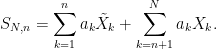
$\displaystyle S_{N,n}=\sum_{k=1}^{n}a_k\tilde X_k+\sum_{k=n+1}^N a_kX_k.$

If we also consider the same sum with the n‘the term excluded,

$\displaystyle \tilde S_{N,n}=\sum_{k=1}^{n-1}a_k\tilde X_k+\sum_{k=n+1}^N a_kX_k,$

then, assuming that the series ${X,\tilde X}$ are chosen independent of each other, ${\tilde S_{N,n}}$ will be independent of both ${X_n}$ and ${\tilde X_n}$ . So, applying (9),

$\displaystyle \begin{aligned} {\mathbb E}[\lvert S_{N,n}\rvert^p] &={\mathbb E}[\lvert\tilde S_{N,n}+a_n\tilde X_n\rvert^p]\\ &\ge{\mathbb E}[\lvert\tilde S_{N,n}+a_nX_n\rvert^p]\\ &={\mathbb E}[\lvert S_{N,n-1}\rvert^p]. \end{aligned}$

As sums of independent normals are normal, ${S_{N,N}}$ is normal with variance ${\sigma_N^2=\sum_{n=1}^Na_n^2}$ . Also, ${S_N=S_{N,0}}$ , so we obtain

$\displaystyle {\mathbb E}[\lvert S_N\rvert^p]\le{\mathbb E}[\lvert S_{N,N}\rvert^p] =\gamma_p\sigma_N^p\le\gamma_p\lVert a\rVert_2^p.$

Letting N increase to infinity and applying Fatou’s lemma on the left hand side gives the result. ⬜

The optimal left-hand inequality for ${p < 2}$ and right-hand inequality for ${2 < p < 3}$ require some further techniques, as the function in lemma 12 is neither convex nor concave. I refer to the paper Ball, Haagerup, and Distribution Functions for these cases, and also to The optimal constants in Khintchine’s inequality for the case 2 < p < 3.

Finally, using the fact that ${\gamma_p}$ and ${2^{p/2-1}}$ are both less than one on the range ${p < 2}$ , I note that the optimal left-hand inequality is given by theorem 10 as,

$\displaystyle c_p=\min(\gamma_p,2^{p/2-1}).$

However, it is not immediately obvious which of the two terms in the minimum is smaller. Writing

$\displaystyle \gamma_p=2^{\frac p2-1}\frac{2}{\sqrt\pi}\Gamma\left(\frac{p+1}{2}\right),$

we see that we should take ${c_p=2^{p/2-1}}$ whenever

$\displaystyle \Gamma\left(\frac{p+1}{2}\right) > \Gamma(3/2)=\frac12\sqrt\pi.$

By log-convexity, there will be a unique ${p_0 < 2}$ solving ${\Gamma((p_0+1)/2)=\Gamma(3/2)}$ and, hence, the expression for ${c_p}$ can be written more clearly as

$\displaystyle c_p =\begin{cases} 2^{p/2-1},&\textrm{for\ }p\le p_0,\\ \gamma_p,&\textrm{for\ }p_0\le p\le2. \end{cases}$

Solving numerically gives ${p_0\approx1.84742}$ .

9 thoughts on “The Khintchine Inequality”

Data says:

10 August 20 at 1:59 PM

Hi George! You claim that Corollary 9 can be generalized to Hilbert spaces (or more generally, uniformly convex spaces). Do you have a reference of this result? Also, I was wondering if you know about an analogous result for the Bochner space $L^0_H$ of equivalence classes of Hilbert space valued random elements?

Thanks for yet another interesting blog entry!

1. George Lowther says:
  
  10 August 20 at 7:01 PM
  
  No reference, this is something I came up with while writing the post. Actually, I did consider if the result holds for all reflexive Banach spaces. Maybe it does, but I am not sure, and did not want to spend too long on what was a side-comment and not the focus of the post. For a Hilbert space it is easy. If the norm of elements of the set $S=\{r_1z_1+\cdots+r_nz_n\colon r\in\{\pm1\}^n\}$ is bounded by K, then
  
  $\displaystyle \sum_{k=1}^n\lVert z_k\rVert^2=2^{-n}\sum_{r\in\{\pm1\}^n}\lVert r_1z_1+\cdots+r_nz_n\rVert^2\le K^2$
  
  and it follows that $\lVert z_k\rVert\to0$ . Uniformly convex spaces are a little trickier. Consider $S_n=\sum_{k=1}^nr_kz_k$ , where $r_n\in\{\pm1\}$ are chosen inductively to maximize $\lVert S_n\rVert$ (given the values of $r_k$ for k less than n). It can be seen that $\lVert S_n\rVert$ is non-decreasing and, as it is bounded by assumption, tends to a limit K (we have not used uniform convexity yet…). The uniform convex property can be used to show that for each fixed positive $\epsilon$ , there exists a $\delta > 0$ such that
  
  $\displaystyle \lVert S_n\rVert = \frac12\lVert(S_n+z_{n+1})+(S_n-z_{n+1})\rVert\le K -\delta$
  
  whenever $\lVert z_{n+1}\rVert > \epsilon$ , which is a contradiction unless $\lVert z_n\rVert < \epsilon$ for all large n, showing that it converges to zero.
  
  It extends to Bochner spaces (defined wrt a Hilbert space H), you can generalise the Khintchine inequality to a_n lying in an arbitrary Hilbert space, so the result should still hold.
  
  1. Data says:
    
    10 August 20 at 10:21 PM
    
    Indeed you are right! Thanks for this nice proof and your insight into these special cases!
    
    In your second equation line, where you bound the sum by $K^2$, should not the first equality be replaced by an inequality? Since you take the sum over all permutations of +-1, you will get some extra terms. Of course, this will change nothing and your elegant argument still holds.
    
    1. George Lowther says:
      
      11 August 20 at 8:16 AM
      
      No, it should be an equality, basically it is the parallelogram law extended to arbitrarily many terms, and is an identity in any Hilbert space.
Richard Guo says:

22 August 20 at 4:08 AM

Thanks for another nice post!

Two minor typos:
(1) Proof of lemma 4: inequality should be reversed before “contradicting (3)”.
(2) Proof of lemma 5: the last inequality should be reversed… and it seems the coefficient before $-\sum_{n} a_n^4$ should be 2?

[George: Fixed, thanks!]

Pingback: Closed form for a minimum related to Khintchine inequality ~ Mathematics ~ mathubs.com
Liekkas says:

27 April 22 at 7:58 PM

I’m sorry, but I don’t think the proof to the right hand side of Theorem 1 is right. The term $\Vert a \Vert_2$ is over an exponential term, how does dividing $\lambda^p$ implies the inequality?

1. George Lowther says:
  
  27 April 22 at 9:06 PM
  
  I mean, lambda is an arbitrary positive number, so can be replaced by lambda / ||a||_2, in which case you get the required inequality.
  
Jonas says:

14 October 22 at 4:06 PM

Thank you for this post! I just used your Lemma 2 and the proof therein to upper bound unknown moments of a non-negative random variable via an interpolation of the moments that I know. This saved a proof within the last hours before submitting an article 🙂

	Harry on Filtrations and Adapted P…
	Anonymous on Analytic Sets
	Daniel on Analytic Sets
	Sid on Martingale Convergence
	northwiz on Preservation of the Local Mart…
	George Lowther on Martingale Convergence
	Sid on Martingale Convergence
	George Lowther on The Burkholder-Davis-Gundy Ine…
	George Lowther on Preservation of the Local Mart…
	northwiz on Preservation of the Local Mart…

The Khintchine Inequality

Optimal Khintchine Constants

Published by George Lowther

9 thoughts on “The Khintchine Inequality”

Leave a Reply Cancel reply

Optimal Khintchine Constants

Like this:

Related

Published by George Lowther

9 thoughts on “The Khintchine Inequality”

Leave a Reply Cancel reply