
A martingale is a stochastic process which stays the same, on average. That is, the expected future value conditional on the present is equal to the current value. Examples include the wealth of a gambler as a function of time, assuming that he is playing a fair game. The canonical example of a continuous time martingale is Brownian motion and, in discrete time, a symmetric random walk is a martingale. As always, we work with respect to a filtered probability space 


![{{\mathbb E}[\vert X_t\vert]<\infty}](https://s0.wp.com/latex.php?latex=%7B%7B%5Cmathbb+E%7D%5B%5Cvert+X_t%5Cvert%5D%3C%5Cinfty%7D&bg=ffffff&fg=000000&s=0&c=20201002)
Definition 1 A martingale,
for all
.
![\displaystyle X_s={\mathbb E}[X_t\mid\mathcal{F}_s]](https://s0.wp.com/latex.php?latex=%5Cdisplaystyle++X_s%3D%7B%5Cmathbb+E%7D%5BX_t%5Cmid%5Cmathcal%7BF%7D_s%5D+&bg=ffffff&fg=000000&s=0&c=20201002)
A closely related concept is that of a submartingale, which is a process which increases on average. This could represent the wealth of a gambler who is involved in games where the odds are in his favour. Similarly, a supermartingale decreases on average.
Definition 2 A process
- submartingale if it is integrable and
for all
- supermartingale if it is integrable and
for all
![\displaystyle X_s\le{\mathbb E}[X_t\mid\mathcal{F}_s]](https://s0.wp.com/latex.php?latex=%5Cdisplaystyle++X_s%5Cle%7B%5Cmathbb+E%7D%5BX_t%5Cmid%5Cmathcal%7BF%7D_s%5D+&bg=ffffff&fg=000000&s=0&c=20201002)
![\displaystyle X_s\ge{\mathbb E}[X_t\mid\mathcal{F}_s]](https://s0.wp.com/latex.php?latex=%5Cdisplaystyle++X_s%5Cge%7B%5Cmathbb+E%7D%5BX_t%5Cmid%5Cmathcal%7BF%7D_s%5D+&bg=ffffff&fg=000000&s=0&c=20201002)
This terminology can perhaps be a bit confusing, but it is related to the result that if 


Clearly, 
Lemma 3 If
is a convex function such that
is integrable, then,
Proof: This is a direct consequence of Jensen’s inequality,
![\displaystyle {\mathbb E}[f(X_t)\mid\mathcal{F}_s]\ge f({\mathbb E}[X_t\mid\mathcal{F}_s])=f(X_s).](https://s0.wp.com/latex.php?latex=%5Cdisplaystyle++%7B%5Cmathbb+E%7D%5Bf%28X_t%29%5Cmid%5Cmathcal%7BF%7D_s%5D%5Cge+f%28%7B%5Cmathbb+E%7D%5BX_t%5Cmid%5Cmathcal%7BF%7D_s%5D%29%3Df%28X_s%29.+&bg=ffffff&fg=000000&s=0&c=20201002) |
⬜
In particular, if 


Lemma 4 Suppose that
Proof: Again, Jensen’s inequality gives the result,
![\displaystyle {\mathbb E}[f(X_t)\mid\mathcal{F}_s]\ge f({\mathbb E}[X_t\mid\mathcal{F}_s])\ge f(X_s),](https://s0.wp.com/latex.php?latex=%5Cdisplaystyle++%7B%5Cmathbb+E%7D%5Bf%28X_t%29%5Cmid%5Cmathcal%7BF%7D_s%5D%5Cge+f%28%7B%5Cmathbb+E%7D%5BX_t%5Cmid%5Cmathcal%7BF%7D_s%5D%29%5Cge+f%28X_s%29%2C+&bg=ffffff&fg=000000&s=0&c=20201002) |
where the final inequality follows from the monotonicity of
So, the positive part 
Elementary integrals
Martingales and submartingales are especially well behaved under stochastic integration. An elementary or elementary predictable process is of the form
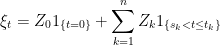 |
(1) |
for 


Stochastic integrals of such elementary processes can be written out explicitly. The integral of the process given by (1) with respect to a stochastic process
 |
The integral over a finite range ![{[0,t]}](https://s0.wp.com/latex.php?latex=%7B%5B0%2Ct%5D%7D&bg=ffffff&fg=000000&s=0&c=20201002)
 |
Note that, for this expression to make sense, it is only strictly necessary for 


Letting 


These elementary integrals satisfy some basic properties which follow directly from the definitions. Linearity in both the integrand 

 |
In differential notation, this is simply 

 |
(2) |
The full theory of stochastic calculus extends these elementary integrals to arbitrary predictable integrands. However, just the elementary case defined above is enough to get going with. First, considering expectations of stochastic integrals leads to the following alternative definition of martingales and submartingales.
Theorem 5 An adapted integrable process
- a martingale if and only if
for all bounded elementary processes
- a submartingale if and only if
(3) for all nonnegative bounded elementary processes
![\displaystyle {\mathbb E}\left[\int_0^\infty \xi\,dX\right]=0](https://s0.wp.com/latex.php?latex=%5Cdisplaystyle++%7B%5Cmathbb+E%7D%5Cleft%5B%5Cint_0%5E%5Cinfty+%5Cxi%5C%2CdX%5Cright%5D%3D0+&bg=ffffff&fg=000000&s=0&c=20201002)
![\displaystyle {\mathbb E}\left[\int_0^\infty\xi\,dX\right]\ge0](https://s0.wp.com/latex.php?latex=%5Cdisplaystyle++%7B%5Cmathbb+E%7D%5Cleft%5B%5Cint_0%5E%5Cinfty%5Cxi%5C%2CdX%5Cright%5D%5Cge0+&bg=ffffff&fg=000000&s=0&c=20201002)
Proof: It is enough to prove the second statement, because the first one follows immediately from applying this to both
![\displaystyle {\mathbb E}\left[\int_0^\infty\xi\,dX\right] = \sum_{k=1}^n{\mathbb E}\left[Z_k(X_{t_k}-X_{s_k})\right] =\sum_{k=1}^n{\mathbb E}\left[Z_k({\mathbb E}[X_{t_k}\mid\mathcal{F}_{s_k}]-X_{s_k})\right]\ge 0.](https://s0.wp.com/latex.php?latex=%5Cdisplaystyle++%7B%5Cmathbb+E%7D%5Cleft%5B%5Cint_0%5E%5Cinfty%5Cxi%5C%2CdX%5Cright%5D+%3D+%5Csum_%7Bk%3D1%7D%5En%7B%5Cmathbb+E%7D%5Cleft%5BZ_k%28X_%7Bt_k%7D-X_%7Bs_k%7D%29%5Cright%5D+%3D%5Csum_%7Bk%3D1%7D%5En%7B%5Cmathbb+E%7D%5Cleft%5BZ_k%28%7B%5Cmathbb+E%7D%5BX_%7Bt_k%7D%5Cmid%5Cmathcal%7BF%7D_%7Bs_k%7D%5D-X_%7Bs_k%7D%29%5Cright%5D%5Cge+0.+&bg=ffffff&fg=000000&s=0&c=20201002) |
Conversely, suppose that inequality (3) holds. Choosing any 
![\displaystyle {\mathbb E}\left[1_A(X_t-X_s)\right]={\mathbb E}\left[\int_0^\infty\xi\,dX\right]\ge 0.](https://s0.wp.com/latex.php?latex=%5Cdisplaystyle++%7B%5Cmathbb+E%7D%5Cleft%5B1_A%28X_t-X_s%29%5Cright%5D%3D%7B%5Cmathbb+E%7D%5Cleft%5B%5Cint_0%5E%5Cinfty%5Cxi%5C%2CdX%5Cright%5D%5Cge+0.+&bg=ffffff&fg=000000&s=0&c=20201002) |
Choosing ![{A=\{{\mathbb E}[X_t\mid\mathcal{F}_s]<X_s\}}](https://s0.wp.com/latex.php?latex=%7BA%3D%5C%7B%7B%5Cmathbb+E%7D%5BX_t%5Cmid%5Cmathcal%7BF%7D_s%5D%3CX_s%5C%7D%7D&bg=ffffff&fg=000000&s=0&c=20201002)
![\displaystyle 0\ge{\mathbb E}\left[\min({\mathbb E}[X_t\mid\mathcal{F}_s]-X_s,0)\right]={\mathbb E}[1_A(X_t-X_s)]\ge 0.](https://s0.wp.com/latex.php?latex=%5Cdisplaystyle++0%5Cge%7B%5Cmathbb+E%7D%5Cleft%5B%5Cmin%28%7B%5Cmathbb+E%7D%5BX_t%5Cmid%5Cmathcal%7BF%7D_s%5D-X_s%2C0%29%5Cright%5D%3D%7B%5Cmathbb+E%7D%5B1_A%28X_t-X_s%29%5D%5Cge+0.+&bg=ffffff&fg=000000&s=0&c=20201002) |
Any non-positive random variable whose expectation is zero must itself be equal to zero, almost surely. So, ![{{\mathbb E}[X_t\mid\mathcal{F}_s]\ge X_s}](https://s0.wp.com/latex.php?latex=%7B%7B%5Cmathbb+E%7D%5BX_t%5Cmid%5Cmathcal%7BF%7D_s%5D%5Cge+X_s%7D&bg=ffffff&fg=000000&s=0&c=20201002)
Elementary integrals preserve the martingale property.
Lemma 6 Let
. Then
- If
.
- If
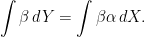
Proof: The first statement follows from the second applied to both 
![\displaystyle {\mathbb E}\left[\int_0^\infty\alpha\,dY\right]={\mathbb E}\left[\int_0^\infty\alpha\xi\,dX\right]\ge 0.](https://s0.wp.com/latex.php?latex=%5Cdisplaystyle++%7B%5Cmathbb+E%7D%5Cleft%5B%5Cint_0%5E%5Cinfty%5Calpha%5C%2CdY%5Cright%5D%3D%7B%5Cmathbb+E%7D%5Cleft%5B%5Cint_0%5E%5Cinfty%5Calpha%5Cxi%5C%2CdX%5Cright%5D%5Cge+0.+&bg=ffffff&fg=000000&s=0&c=20201002) |
This inequality follows from the previous lemma and, again by the previous lemma, it shows that
Finally, optional stopping of martingales follows from the properties of elementary integrals. This extends the martingale property to random stopping times. The value 

 |
is elementary and, furthermore, equation (2) can be extended to give
 |
The optional stopping theorem states that the class of martingales is closed under stopping at arbitrary stopping times.
Lemma 7 Let
is also a martingale (resp. submartingale, supermartingale).
Proof: This follows from applying Lemma 6 to the following identity
 |
⬜

Hello George, I really like this blog.
Do you know whether the Theorem 5 result![E\left[\int_0^t \xi\,dW\right]=0](https://s0.wp.com/latex.php?latex=E%5Cleft%5B%5Cint_0%5Et+%5Cxi%5C%2CdW%5Cright%5D%3D0&bg=ffffff&fg=000000&s=0&c=20201002) , for
, for  a martingale, can be extended to a more general class of stochastic processes
  ? Maybe something like
  being integrable, adapted to the natural filtration of
  , a.s. cadlag and a.s. uniformly bounded on
 ![[0,t]](https://s0.wp.com/latex.php?latex=%5B0%2Ct%5D&bg=ffffff&fg=000000&s=0&c=20201002) ?
?
Yes you can, but you probably want to at least be predictable, and you need to first develop some theory in order to give meaning to the integral, and impose sufficient conditions on the sample paths of W. The point of this post is that we do not require any prior knowledge of stochastic integration nor that we have well-behaved versions (such as right-continuous) of the process W.
Hi George when you define simple stopping time at the bottom, do you take t_0 = 0? In the sum there should be a t_0. But in this case what happens if \tau takes 0? By definition you have it should be t_1 = 0. Also in Lemma 7, why is there X_0 in addition to the integral for X^\tau?
Yes, I took t_0=0. I edited the post to clarify. It should be fine when tau is zero.
In lemma 7 I added on X_0 because, by definition, the integral over an interval (0,t] is X_t-X_0, so need to add this term back on.
Hi, in the proof of Theorem 5, the last part of the first equation reads![\displaystyle \sum_{k=1}^n{\mathbb E}\left[Z_k({\mathbb E}[X_{t_k}\mid\mathcal{F}_{s_k}]-X_s)\right]\ge 0](https://s0.wp.com/latex.php?latex=%5Cdisplaystyle+%5Csum_%7Bk%3D1%7D%5En%7B%5Cmathbb+E%7D%5Cleft%5BZ_k%28%7B%5Cmathbb+E%7D%5BX_%7Bt_k%7D%5Cmid%5Cmathcal%7BF%7D_%7Bs_k%7D%5D-X_s%29%5Cright%5D%5Cge+0&bg=ffffff&fg=000000&s=0&c=20201002) . Shouldn’t the last
. Shouldn’t the last  be
be  ?
?
Fixed. Thanks!