Pathwise Martingale Inequalities

Recall Doob’s inequalities, covered earlier in these notes, which bound expectations of functions of the maximum of a martingale in terms of its terminal distribution. Although these are often applied to martingales, they hold true more generally for cadlag submartingales. Here, I use ${\bar X_t\equiv\sup_{s\le t}X_s}$ to denote the running maximum of a process.

Theorem 1 Let X be a nonnegative cadlag submartingale. Then,

${{\mathbb P}\left(\bar X_t \ge K\right)\le K^{-1}{\mathbb E}[X_t]}$ for all ${K > 0}$ .

${\lVert\bar X_t\rVert_p\le (p/(p-1))\lVert X_t\rVert_p}$ for all ${p > 1}$ .

${{\mathbb E}[\bar X_t]\le(e/(e-1)){\mathbb E}[X_t\log X_t+1]}$ .

In particular, for a cadlag martingale X, then ${\lvert X\rvert}$ is a submartingale, so theorem 1 applies with ${\lvert X\rvert}$ in place of X.

We also saw the following much stronger (sub)martingale inequality in the post on the maximum maximum of martingales with known terminal distribution.

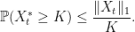
Theorem 2 Let X be a cadlag submartingale. Then, for any real K and nonnegative real t,

$\displaystyle {\mathbb P}(\bar X_t\ge K)\le\inf_{x < K}\frac{{\mathbb E}[(X_t-x)_+]}{K-x}.$ (1)

This is particularly sharp, in the sense that for any distribution for ${X_t}$ , there exists a martingale with this terminal distribution for which (1) becomes an equality simultaneously for all values of K. Furthermore, all of the inequalities stated in theorem 1 follow from (1). For example, the first one is obtained by taking ${x=0}$ in (1). The remaining two can also be proved from (1) by integrating over K.

Note that all of the submartingale inequalities above are of the form

$\displaystyle {\mathbb E}[F(\bar X_t)]\le{\mathbb E}[G(X_t)]$

(2)

for certain choices of functions ${F,G\colon{\mathbb R}\rightarrow{\mathbb R}^+}$ . The aim of this post is to show how they have a more general `pathwise’ form,

$\displaystyle F(\bar X_t)\le G(X_t) - \int_0^t\xi\,dX$

(3)

for some nonnegative predictable process ${\xi}$ . It is relatively straightforward to show that (2) follows from (3) by noting that the integral is a submartingale and, hence, has nonnegative expectation. To be rigorous, there are some integrability considerations to deal with, so a proof will be included later in this post.

Inequality (3) is required to hold almost everywhere, and not just in expectation, so is a considerably stronger statement than the standard martingale inequalities. Furthermore, it is not necessary for X to be a submartingale for (3) to make sense, as it holds for all semimartingales. We can go further, and even drop the requirement that X is a semimartingale. As we will see, in the examples covered in this post, ${\xi_t}$ will be of the form ${h(\bar X_{t-})}$ for an increasing right-continuous function ${h\colon{\mathbb R}\rightarrow{\mathbb R}}$ , so integration by parts can be used,

$\displaystyle \int h(\bar X_-)\,dX = h(\bar X)X-h(\bar X_0)X_0 - \int X\,dh(\bar X).$

(4)

The right hand side of (4) is well-defined for any cadlag real-valued process, by using the pathwise Lebesgue–Stieltjes integral with respect to the increasing process ${h(\bar X)}$ , so can be used as the definition of ${\int h(\bar X_-)dX}$ . In the case where X is a semimartingale, integration by parts ensures that this agrees with the stochastic integral ${\int\xi\,dX}$ . Since we now have an interpretation of (3) in a pathwise sense for all cadlag processes X, it is no longer required to suppose that X is a submartingale, a semimartingale, or even require the existence of an underlying probability space. All that is necessary is for ${t\mapsto X_t}$ to be a cadlag real-valued function. Hence, we reduce the martingale inequalities to straightforward results of real-analysis not requiring any probability theory and, consequently, are much more general. I state the precise pathwise generalizations of Doob’s inequalities now, leaving the proof until later in the post. As the first of inequality of theorem 1 is just the special case of (1) with ${x=0}$ , we do not need to explicitly include this here.

Theorem 3 Let X be a cadlag process and t be a nonnegative time.

For real ${K > x}$ ,

$\displaystyle 1_{\{\bar X_t\ge K\}}\le\frac{(X_t-x)_+}{K-x}-\int_0^t\xi\,dX$ (5)

where ${\xi=(K-x)^{-1}1_{\{\bar X_-\ge K\}}}$ .

If X is nonnegative and p,q are positive reals with ${p^{-1}+q^{-1}=1}$ then,

$\displaystyle \bar X_t^p\le q^p X^p_t-\int_0^t\xi dX$ (6)

where ${\xi=pq\bar X_-^{p-1}}$ .

If X is nonnegative then,

$\displaystyle \bar X_t\le\frac{e}{e-1}\left( X_t \log X_t +1\right)-\int_0^t\xi\,dX$ (7)

where ${\xi=\frac{e}{e-1}\log(\bar X_-\vee1)}$ .

Continue reading “Pathwise Martingale Inequalities” →

The Maximum Maximum of Martingales with Known Terminal Distribution

In this post I will be concerned with the following problem — given a martingale X for which we know the distribution at a fixed time, and we are given nothing else, what is the best bound we can obtain for the maximum of X up until that time? This is a question with a long history, starting with Doob’s inequalities which bound the maximum in the ${L^p}$ norms and in probability. Later, Blackwell and Dubins (3), Dubins and Gilat (5) and Azema and Yor (1,2) showed that the maximum is bounded above, in stochastic order, by the Hardy-Littlewood transform of the terminal distribution. Furthermore, this bound is the best possible in the sense that there do exists martingales for which it can be attained, for any permissible terminal distribution. Hobson (7,8) considered the case where the starting law is also known, and this was further generalized to the case with a specified distribution at an intermediate time by Brown, Hobson and Rogers (4). Finally, Henry-Labordère, Obłój, Spoida and Touzi (6) considered the case where the distribution of the martingale is specified at an arbitrary set of times. In this post, I will look at the case where only the terminal distribution is specified. This leads to interesting constructions of martingales and, in particular, of continuous martingales with specified terminal distributions, with close connections to the Skorokhod embedding problem.

I will be concerned with the maximum process of a cadlag martingale X,

$\displaystyle X^*_t=\sup_{s\le t}X_s,$

which is increasing and adapted. We can state and prove the bound on ${X^*}$ relatively easily, although showing that it is optimal is more difficult. As the result holds more generally for submartingales, I state it in this case, although I am more concerned with martingales here.

Theorem 1 If X is a cadlag submartingale then, for each ${t\ge0}$ and ${x\in{\mathbb R}}$ ,

$\displaystyle {\mathbb P}\left(X^*_t\ge x\right)\le\inf_{y < x}\frac{{\mathbb E}\left[(X_t-y)_+\right]}{x-y}.$ (1)

Proof: We just need to show that the inequality holds for each ${y < x}$ , and then it immediately follows for the infimum. Choosing ${y < x^\prime < x}$ , consider the stopping time

$\displaystyle \tau=\inf\{s\ge0\colon X_s\ge x^\prime\}.$

Then, ${\tau \le t}$ and ${X_\tau\ge x^\prime}$ whenever ${X^*_t \ge x}$ . As ${f(z)\equiv(z-y)_+}$ is nonnegative and increasing in z, this means that ${1_{\{X^*_t\ge x\}}}$ is bounded above by ${f(X_{\tau\wedge t})/f(x^\prime)}$ . Taking expectations,

$\displaystyle {\mathbb P}\left(X^*_t\ge x\right)\le{\mathbb E}\left[f(X_{\tau\wedge t})\right]/f(x^\prime).$

Since f is convex and increasing, ${f(X)}$ is a submartingale so, using optional sampling,

$\displaystyle {\mathbb P}\left(X^*_t\ge x\right)\le{\mathbb E}\left[f(X_t)\right]/f(x^\prime).$

Letting ${x^\prime}$ increase to ${x}$ gives the result. ⬜

The bound stated in Theorem 1 is also optimal, and can be achieved by a continuous martingale. In this post, all measures on ${{\mathbb R}}$ are defined with respect to the Borel sigma-algebra.

Theorem 2 If ${\mu}$ is a probability measure on ${{\mathbb R}}$ with ${\int\lvert x\rvert\,d\mu(x) < \infty}$ and ${t > 0}$ then there exists a continuous martingale X (defined on some filtered probability space) such that ${X_t}$ has distribution ${\mu}$ and (1) is an equality for all ${x\in{\mathbb R}}$ .

Continue reading “The Maximum Maximum of Martingales with Known Terminal Distribution” →

Rao’s Quasimartingale Decomposition

In this post I’ll give a proof of Rao’s decomposition for quasimartingales. That is, every quasimartingale decomposes as the sum of a submartingale and a supermartingale. Equivalently, every quasimartingale is a difference of two submartingales, or alternatively, of two supermartingales. This was originally proven by Rao (Quasi-martingales, 1969), and is an important result in the general theory of continuous-time stochastic processes.

As always, we work with respect to a filtered probability space ${(\Omega,\mathcal{F},\{\mathcal{F}_t\}_{t\ge0},{\mathbb P})}$ . It is not required that the filtration satisfies either of the usual conditions — the filtration need not be complete or right-continuous. The methods used in this post are elementary, requiring only basic measure theory along with the definitions and first properties of martingales, submartingales and supermartingales. Other than referring to the definitions of quasimartingales and mean variation given in the previous post, there is no dependency on any of the general theory of semimartingales, nor on stochastic integration other than for elementary integrands.

Recall that, for an adapted integrable process X, the mean variation on an interval ${[0,t]}$ is

$\displaystyle {\rm Var}_t(X)=\sup{\mathbb E}\left[\int_0^t\xi\,dX\right],$

where the supremum is taken over all elementary processes ${\xi}$ with ${\vert\xi\vert\le1}$ . Then, X is a quasimartingale if and only if ${{\rm Var}_t(X)}$ is finite for all positive reals t. It was shown that all supermartingales are quasimartingales with mean variation given by

$\displaystyle {\rm Var}_t(X)={\mathbb E}\left[X_0-X_t\right].$

(1)

Rao’s decomposition can be stated in several different ways, depending on what conditions are required to be satisfied by the quasimartingale X. As the definition of quasimartingales does differ between texts, there are different versions of Rao’s theorem around although, up to martingale terms, they are equivalent. In this post, I’ll give three different statements with increasingly stronger conditions for X. First, the following statement applies to all quasimartingales as defined in these notes. Theorem 1 can be compared to the Jordan decomposition, which says that any function ${f\colon{\mathbb R}_+\rightarrow{\mathbb R}}$ with finite variation on bounded intervals can be decomposed as the difference of increasing functions or, equivalently, of decreasing functions. Replacing finite variation functions by quasimartingales and decreasing functions by supermartingales gives the following.

Theorem 1 (Rao) A process X is a quasimartingale if and only if it decomposes as

$\displaystyle X=Y-Z$ (2)

for supermartingales Y and Z. Furthermore,

this decomposition can be done in a minimal sense, so that if ${X=Y^\prime-Z^\prime}$ is any other such decomposition then ${Y^\prime-Y=Z^\prime-Z}$ is a supermartingale.

the inequality

$\displaystyle {\rm Var}_t(X)\le{\mathbb E}[Y_0-Y_t]+{\mathbb E}[Z_0-Z_t],$ (3)

holds, with equality for all ${t\ge0}$ if and only if the decomposition is minimal.

the minimal decomposition is unique up to a martingale. That is, if ${X=Y-Z=Y^\prime-Z^\prime}$ are two such minimal decompositions, then ${Y^\prime-Y=Z^\prime-Z}$ is a martingale.

Continue reading “Rao’s Quasimartingale Decomposition” →

Quasimartingales

Quasimartingales are a natural generalization of martingales, submartingales and supermartingales. They were first introduced by Fisk in order to extend the Doob-Meyer decomposition to a larger class of processes, showing that continuous quasimartingales can be decomposed into martingale and finite variation terms (Quasi-martingales, 1965). This was later extended to right-continuous processes by Orey (F-Processes, 1967). The way in which quasimartingales relate to sub- and super-martingales is very similar to how functions of finite variation relate to increasing and decreasing functions. In particular, by the Jordan decomposition, any finite variation function on an interval decomposes as the sum of an increasing and a decreasing function. Similarly, a stochastic process is a quasimartingale if and only if it can be written as the sum of a submartingale and a supermartingale. This important result was first shown by Rao (Quasi-martingales, 1969), and means that much of the theory of submartingales can be extended without much work to also cover quasimartingales.

Often, given a process, it is important to show that it is a semimartingale so that the techniques of stochastic calculus can be applied. If there is no obvious decomposition into local martingale and finite variation terms, then, one way of doing this is to show that it is a quasimartingale. All right-continuous quasimartingales are semimartingales. This result is also important in the general theory of semimartingales with, for example, many proofs of the Bichteler-Dellacherie theorem involving quasimartingales.

In this post, I will mainly be concerned with the definition and very basic properties of quasimartingales, and look at the more advanced theory in the following post. We work with respect to a filtered probability space ${(\Omega,\mathcal{F},\{\mathcal{F}_t\}_{t\ge0},{\mathbb P})}$ . It is not necessary to assume that either of the usual conditions, of right-continuity or completeness, hold. First, the mean variation of a process is defined as follows.

Definition 1 The mean variation of an integrable stochastic process X on an interval ${[0,t]}$ is

$\displaystyle {\rm Var}_t(X)=\sup{\mathbb E}\left[\sum_{k=1}^n\left\vert{\mathbb E}\left[X_{t_k}-X_{t_{k-1}}\;\vert\mathcal{F}_{t_{k-1}}\right]\right\vert\right].$ (1)

Here, the supremum is taken over all finite sequences of times,

$\displaystyle 0=t_0\le t_1\le\cdots\le t_n=t.$

A quasimartingale, then, is a process with finite mean variation on each bounded interval.

Definition 2 A quasimartingale, X, is an integrable adapted process such that ${{\rm Var}_t(X)}$ is finite for each time ${t\in{\mathbb R}_+}$ .

Continue reading “Quasimartingales” →

The Doob-Meyer Decomposition

The Doob-Meyer decomposition was a very important result, historically, in the development of stochastic calculus. This theorem states that every cadlag submartingale uniquely decomposes as the sum of a local martingale and an increasing predictable process. For one thing, if X is a square-integrable martingale then Jensen’s inequality implies that ${X^2}$ is a submartingale, so the Doob-Meyer decomposition guarantees the existence of an increasing predictable process ${\langle X\rangle}$ such that ${X^2-\langle X\rangle}$ is a local martingale. The term ${\langle X\rangle}$ is called the predictable quadratic variation of X and, by using a version of the Ito isometry, can be used to define stochastic integration with respect to square-integrable martingales. For another, semimartingales were historically defined as sums of local martingales and finite variation processes, so the Doob-Meyer decomposition ensures that all local submartingales are also semimartingales. Going further, the Doob-Meyer decomposition is used as an important ingredient in many proofs of the Bichteler-Dellacherie theorem.

The approach taken in these notes is somewhat different from the historical development, however. We introduced stochastic integration and semimartingales early on, without requiring much prior knowledge of the general theory of stochastic processes. We have also developed the theory of semimartingales, such as proving the Bichteler-Dellacherie theorem, using a stochastic integration based method. So, the Doob-Meyer decomposition does not play such a pivotal role in these notes as in some other approaches to stochastic calculus. In fact, the special semimartingale decomposition already states a form of the Doob-Meyer decomposition in a more general setting. So, the main part of the proof given in this post will be to show that all local submartingales are semimartingales, allowing the decomposition for special semimartingales to be applied.

The Doob-Meyer decomposition is especially easy to understand in discrete time, where it reduces to the much simpler Doob decomposition. If ${\{X_n\}_{n=0,1,2,\ldots}}$ is an integrable discrete-time process adapted to a filtration ${\{\mathcal{F}_n\}_{n=0,1,2,\ldots}}$ , then the Doob decomposition expresses X as

$\displaystyle \setlength\arraycolsep{2pt} \begin{array}{rl} \displaystyle X_n&\displaystyle=M_n+A_n,\smallskip\\ \displaystyle A_n&\displaystyle=\sum_{k=1}^n{\mathbb E}\left[X_k-X_{k-1}\;\vert\mathcal{F}_{k-1}\right]. \end{array}$

(1)

As previously discussed, M is then a martingale and A is an integrable process which is also predictable, in the sense that ${A_n}$ is ${\mathcal{F}_{n-1}}$ -measurable for each ${n > 0}$ . Furthermore, X is a submartingale if and only if ${{\mathbb E}[X_n-X_{n-1}\vert\mathcal{F}_{n-1}]\ge0}$ or, equivalently, if A is almost surely increasing.

Moving to continuous time, we work with respect to a complete filtered probability space ${(\Omega,\mathcal{F},\{\mathcal{F}_t\}_{t\ge0},{\mathbb P})}$ with time index t ranging over the nonnegative real numbers. Then, the continuous-time version of (1) takes A to be a right-continuous and increasing process which is predictable, in the sense that it is measurable with respect to the σ-algebra generated by the class of left-continuous and adapted processes. Often, the Doob-Meyer decomposition is stated under additional assumptions, such as X being of class (D) or satisfying some similar uniform integrability property. To be as general possible, the statement I give here only requires X to be a local submartingale, and furthermore states how the decomposition is affected by various stronger hypotheses that X may satisfy.

Theorem 1 (Doob-Meyer) Any local submartingale X has a unique decomposition

$\displaystyle X=M+A,$ (2)

where M is a local martingale and A is a predictable increasing process starting from zero.

Furthermore,

if X is a proper submartingale, then A is integrable and satisfies

$\displaystyle {\mathbb E}[A_\tau]\le{\mathbb E}[X_\tau-X_0]$ (3)

for all uniformly bounded stopping times ${\tau}$ .

X is of class (DL) if and only if M is a proper martingale and A is integrable, in which case

$\displaystyle {\mathbb E}[A_\tau]={\mathbb E}[X_\tau-X_0]$ (4)

for all uniformly bounded stopping times ${\tau}$ .

X is of class (D) if and only if M is a uniformly integrable martingale and ${A_\infty}$ is integrable. Then, ${X_\infty=\lim_{t\rightarrow\infty}X_t}$ and ${M_\infty=\lim_{t\rightarrow\infty}M_t}$ exist almost surely, and (4) holds for all (not necessarily finite) stopping times ${\tau}$ .

Continue reading “The Doob-Meyer Decomposition” →

Local Martingales

Recall from the previous post that a cadlag adapted process ${X}$ is a local martingale if there is a sequence ${\tau_n}$ of stopping times increasing to infinity such that the stopped processes ${1_{\{\tau_n>0\}}X^{\tau_n}}$ are martingales. Local submartingales and local supermartingales are defined similarly.

An example of a local martingale which is not a martingale is given by the `double-loss’ gambling strategy. Interestingly, in 18th century France, such strategies were known as martingales and is the origin of the mathematical term. Suppose that a gambler is betting sums of money, with even odds, on a simple win/lose game. For example, betting that a coin toss comes up heads. He could bet one dollar on the first toss and, if he loses, double his stake to two dollars for the second toss. If he loses again, then he is down three dollars and doubles the stake again to four dollars. If he keeps on doubling the stake after each loss in this way, then he is always gambling one more dollar than the total losses so far. He only needs to continue in this way until the coin eventually does come up heads, and he walks away with net winnings of one dollar. This therefore describes a fair game where, eventually, the gambler is guaranteed to win.

Of course, this is not an effective strategy in practise. The losses grow exponentially and, if he doesn’t win quickly, the gambler must hit his credit limit in which case he loses everything. All that the strategy achieves is to trade a large probability of winning a dollar against a small chance of losing everything. It does, however, give a simple example of a local martingale which is not a martingale.

The gamblers winnings can be defined by a stochastic process ${\{Z_n\}_{n=1,\ldots}}$ representing his net gain (or loss) just before the n’th toss. Let ${\epsilon_1,\epsilon_2,\ldots}$ be a sequence of independent random variables with ${{\mathbb P}(\epsilon_n=1)={\mathbb P}(\epsilon_n=-1)=1/2}$ . Here, ${\epsilon_n}$ represents the outcome of the n’th toss, with 1 referring to a head and -1 referring to a tail. Set ${Z_1=0}$ and

$\displaystyle Z_{n}=\begin{cases} 1,&\text{if }Z_{n-1}=1,\\ Z_{n-1}+\epsilon_n(1-Z_{n-1}),&\text{otherwise}. \end{cases}$

This is a martingale with respect to its natural filtration, starting at zero and, eventually, ending up equal to one. It can be converted into a local martingale by speeding up the time scale to fit infinitely many tosses into a unit time interval

$\displaystyle X_t=\begin{cases} Z_n,&\text{if }1-1/n\le t<1-1/(n+1),\\ 1,&\text{if }t\ge 1. \end{cases}$

This is a martingale with respect to its natural filtration on the time interval ${[0,1)}$ . Letting ${\tau_n=\inf\{t\colon\vert X_t\vert\ge n\}}$ then the optional stopping theorem shows that ${X^{\tau_n}_t}$ is a uniformly bounded martingale on ${t<1}$ , continuous at ${t=1}$ , and constant on ${t\ge 1}$ . This is therefore a martingale, showing that ${X}$ is a local martingale. However, ${{\mathbb E}[X_1]=1\not={\mathbb E}[X_0]=0}$ , so it is not a martingale. Continue reading “Local Martingales” →

Localization

Special classes of processes, such as martingales, are very important to the study of stochastic calculus. In many cases, however, processes under consideration `almost’ satisfy the martingale property, but are not actually martingales. This occurs, for example, when taking limits or stochastic integrals with respect to martingales. It is necessary to generalize the martingale concept to that of local martingales. More generally, localization is a method of extending a given property to a larger class of processes. In this post I mention a few definitions and simple results concerning localization, and look more closely at local martingales in the next post.

Definition 1 Let P be a class of stochastic processes. Then, a process X is locally in P if there exists a sequence of stopping times ${\tau_n\uparrow\infty}$ such that the stopped processes

$\displaystyle 1_{\{\tau_n>0\}}X^{\tau_n}$

are in P. The sequence ${\tau_n}$ is called a localizing sequence for X (w.r.t. P).

I write ${P_{\rm loc}}$ for the processes locally in P. Choosing the sequence ${\tau_n\equiv\infty}$ of stopping times shows that ${P\subseteq P_{\rm loc}}$ . A class of processes is said to be stable if ${1_{\{\tau>0\}}X^\tau}$ is in P whenever X is, for all stopping times ${\tau}$ . For example, the optional stopping theorem shows that the classes of cadlag martingales, cadlag submartingales and cadlag supermartingales are all stable.

Definition 2 A process is a

a local martingale if it is locally in the class of cadlag martingales.

a local submartingale if it is locally in the class of cadlag submartingales.

a local supermartingale if it is locally in the class of cadlag supermartingales.

Continue reading “Localization” →

Class (D) Processes

A stochastic process X is said to be uniformly integrable if the set of random variables ${\{X_t\colon t\in{\mathbb R}_+\}}$ is uniformly integrable. However, even if this is the case, it does not follow that the set of values of the process sampled at arbitrary stopping times is uniformly integrable.

For the case of a cadlag martingale X, optional sampling can be used. If ${t\ge 0}$ is any fixed time then this says that ${X_\tau={\mathbb E}[X_t\mid\mathcal{F}_\tau]}$ for stopping times ${\tau\le t}$ . As sets of conditional expectations of a random variable are uniformly integrable, the following result holds.

Lemma 1 Let X be a cadlag martingale. Then, for each ${t\ge 0}$ , the set

$\displaystyle \{X_\tau\colon\tau\le t\text{\ is\ a\ stopping\ time}\}$

is uniformly integrable.

This suggests the following generalized concepts of uniform integrability for stochastic processes.

Definition 2 Let X be a jointly measurable stochastic process. Then, it is

of class (D) if ${\{X_\tau\colon\tau<\infty\text{ is a stopping time}\}}$ is uniformly integrable.

of class (DL) if, for each ${t\ge 0}$ , ${\{X_\tau\colon\tau\le t\text{ is a stopping time}\}}$ is uniformly integrable.

Continue reading “Class (D) Processes” →

Martingale Inequalities

Martingale inequalities are an important subject in the study of stochastic processes. The subject of this post is Doob’s inequalities which bound the distribution of the maximum value of a martingale in terms of its terminal distribution, and is a consequence of the optional sampling theorem. We work with respect to a filtered probability space ${(\Omega,\mathcal{F},\{\mathcal{F}_t\}_{t\ge 0},{\mathbb P})}$ . The absolute maximum process of a martingale is denoted by ${X^*_t\equiv\sup_{s\le t}\vert X_s\vert}$ . For any real number ${p\ge 1}$ , the ${L^p}$ -norm of a random variable ${Z}$ is

$\displaystyle \Vert Z\Vert_p\equiv{\mathbb E}[|Z|^p]^{1/p}.$

Then, Doob’s inequalities bound the distribution of the maximum of a martingale by the ${L^1}$ -norm of its terminal value, and bound the ${L^p}$ -norm of its maximum by the ${L^p}$ -norm of its terminal value for all ${p>1}$ .

Theorem 1 Let ${X}$ be a cadlag martingale and ${t>0}$ . Then

for every ${K>0}$ ,
$\displaystyle {\mathbb P}(X^*_t\ge K)\le\frac{\lVert X_t\rVert_1}{K}.$

for every ${p>1}$ ,
$\displaystyle \lVert X^*_t\rVert_p\le \frac{p}{p-1}\Vert X_t\Vert_p.$

$\displaystyle \lVert X^*_t\rVert_1\le\frac e{e-1}{\mathbb E}\left[\lvert X_t\rvert \log\lvert X_t\rvert+1\right].$

Continue reading “Martingale Inequalities” →

Martingale Convergence

The martingale property is strong enough to ensure that, under relatively weak conditions, we are guaranteed convergence of the processes as time goes to infinity. In a previous post, I used Doob’s upcrossing inequality to show that, with probability one, discrete-time martingales will converge at infinity under the extra condition of ${L^1}$ -boundedness. Here, I consider continuous-time martingales. This is a more general situation, because it considers limits as time runs through the uncountably infinite set of positive reals instead of the countable set of positive integer times. Although these results can also be proven in a similar way by counting the upcrossings of a process, I instead show how they follow directly from the existence of cadlag modifications. We work with respect to a complete filtered probability space ${(\Omega,\mathcal{F},\{\mathcal{F}_t\}_{t\ge 0},{\mathbb P})}$ .

Recall that a stochastic process ${X}$ is ${L^1}$ -bounded if the set ${\{X_t\colon t\in{\mathbb R}_+\}}$ is ${L^1}$ -bounded. That is, ${{\mathbb E}|X_t|}$ is bounded above by some finite value as ${t}$ runs through the positive reals.

Theorem 1 Let ${X}$ be a cadlag and ${L^1}$ -bounded martingale (or submartingale, or supermartingale). Then, the limit ${X_\infty=\lim_{t\rightarrow\infty}X_t}$ exists and is finite, with probability one.

Continue reading “Martingale Convergence” →

	Anonymous on About
	Anonymous on About
	Anonymous on The Stochastic Integral
	Anonymous on Bessel Processes
	Anonymous on Bessel Processes
	Stat Prof on Pathwise Regularity of Optiona…
	Yang Chu on Spitzer’s Formula
	Anonymous on About
	Anonymous on Continuous Processes with Inde…
	Anonymous on Continuous Processes with Inde…