Martingale Inequalities

Martingale inequalities are an important subject in the study of stochastic processes. The subject of this post is Doob’s inequalities which bound the distribution of the maximum value of a martingale in terms of its terminal distribution, and is a consequence of the optional sampling theorem. We work with respect to a filtered probability space ${(\Omega,\mathcal{F},\{\mathcal{F}_t\}_{t\ge 0},{\mathbb P})}$ . The absolute maximum process of a martingale is denoted by ${X^*_t\equiv\sup_{s\le t}\vert X_s\vert}$ . For any real number ${p\ge 1}$ , the ${L^p}$ -norm of a random variable ${Z}$ is

$\displaystyle \Vert Z\Vert_p\equiv{\mathbb E}[|Z|^p]^{1/p}.$

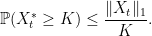
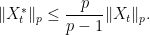
Then, Doob’s inequalities bound the distribution of the maximum of a martingale by the ${L^1}$ -norm of its terminal value, and bound the ${L^p}$ -norm of its maximum by the ${L^p}$ -norm of its terminal value for all ${p>1}$ .

Theorem 1 Let ${X}$ be a cadlag martingale and ${t>0}$ . Then

for every ${K>0}$ ,
$\displaystyle {\mathbb P}(X^*_t\ge K)\le\frac{\lVert X_t\rVert_1}{K}.$

for every ${p>1}$ ,
$\displaystyle \lVert X^*_t\rVert_p\le \frac{p}{p-1}\Vert X_t\Vert_p.$

$\displaystyle \lVert X^*_t\rVert_1\le\frac e{e-1}{\mathbb E}\left[\lvert X_t\rvert \log\lvert X_t\rvert+1\right].$

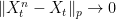
We can define a topology on the space of cadlag martingales so that a sequence ${X^n}$ of martingales converges to a limit ${X}$ if ${\Vert X^n_t-X_t\Vert_p\rightarrow 0}$ as ${n\rightarrow\infty}$ . It is clear that ${\Vert X_t\Vert_p\le\Vert X^*_t\Vert_p}$ for any process and, consequently Doob’s second inequality above shows that this topology is equivalent to the seemingly much stronger condition that ${\Vert(X^n-X)^*_t\Vert_p\rightarrow 0}$ , for any ${p>1}$ .

The second statement above does not extend to ${p=1}$ to give a bound for ${\lVert X^*_t\rVert_1}$ in terms of ${\lVert X_t\rVert_1}$ . Instead, we have the rather weaker third statement above, which requires ${X_t\log\lvert X_t\rvert}$ to be integrable in order to give a nontrivial upper bound. In fact, there exist martingales X such that the maximum ${X^*_t}$ has infinite expectation at all positive times even though, by definition, ${\lVert X_t\rVert_1}$ is finite.

Doob’s martingale inequalities are a consequence of the following inequalities applied to the submartingale ${|X_t|}$ .

Theorem 2 Let ${X}$ be a nonnegative cadlag submartingale. Then,

${{\mathbb P}(X^*_t\ge K)\le \lVert X_t\rVert_1/K}$ for each ${K>0}$ .

${\Vert X^*_t\Vert_p\le(p/(p-1))\Vert X_t\Vert_p}$ for each ${p>1}$ .

${\lVert X^*_t\rVert_1\le(e/(e-1)){\mathbb E}[X_t\log X_t+1]}$ .

I briefly note that the third inequality looks a bit odd, as it is not dimensionally consistent. This means that, unlike the other two, applying it to ${aX}$ for positive a gives a slightly different inequality. Specifically, applying it to ${aX}$ and dividing through by a gives

$\displaystyle \lVert X^*_t\rVert_1\le(e/(e-1)){\mathbb E}[X_t\log X_t+c]$

where c is equal to ${{\mathbb E}[X_t]\log a+1/a}$ . The optimal value occurs at ${a=1/{\mathbb E}[X_t]}$ giving

$\displaystyle \lVert X^*_t\rVert_1\le(e/(e-1))\left({\mathbb E}[X_t\log X_t]+{\mathbb E}[X_t](1-\log{\mathbb E}[X_t])\right).$

This is dimensionally consistent — replacing X by ${aX}$ scales both sides by a. Furthermore, as ${x(1-\log x)}$ is bounded above by 1, it is stronger in this form than as stated in Theorem 2. However, the versions stated above are simpler, and the important thing is that they have the same coefficient for the dominant term ${{\mathbb E}[X_t\log X_t]}$ .

To prove Theorem 2, we start with the following submartingale inequality from which each of Doob’s inequalities will follow.

Lemma 3 Let ${X}$ be a nonnegative cadlag submartingale. Then, for each ${K,t > 0}$ ,

$\displaystyle K{\mathbb P}(X^*_t\ge K)\le{\mathbb E}\left[1_{\{X^*_t\ge K\}}X_t\right].$ (1)

Proof: By completing the filtration if necessary, without loss of generality we assume that it is complete. Consider the first time at which the process reaches a positive value ${L < K}$ ,

$\displaystyle \tau=\inf\left\{t\in{\mathbb R}_+\colon X_t\ge L\right\}$

which, by the debut theorem, is a stopping time. Then ${X_\tau\ge L}$ whenever ${\tau\le t}$ and, ${\{X^*_t\ge K\}\subseteq\{\tau\le t\}}$ . Optional sampling gives

$\displaystyle L1_{\{X^*_t \ge K\}}\le 1_{\{\tau\le t\}}X_\tau \le {\mathbb E}[1_{\{X^*_t\ge L\}}X_t\vert\mathcal{F}_\tau].$

Taking expectations

$\displaystyle L{\mathbb P}(X^*_t\ge K)\le {\mathbb E}[1_{\{X^*_t\ge L\}}X_t],$

and (1) follows by letting L increase to K. ⬜

We use (1) to prove Doob’s inequalities.

Proof of Theorem 2: Bounding the right hand side of (1) by ${{\mathbb E}[X_t]}$ gives the first inequality. Next, for ${p > 1}$ , multiply by ${K^{p-2}}$ and integrate up to a limit ${L>0}$ to get,

$\displaystyle \setlength\arraycolsep{2pt} \begin{array}{rcl} \displaystyle{\mathbb E}\left[(L\wedge X^*_t)^p\right] &\displaystyle=&\displaystyle p{\mathbb E}\left[\int_0^L K^{p-1} 1_{\{X^*_t\ge K\}}\,dK\right]\smallskip\\ &\displaystyle=&\displaystyle p\int_0^L K^{p-1}{\mathbb P}(X^*_t\ge K)\,dK\smallskip\\ &\displaystyle\le &\displaystyle p\int_0^L K^{p-2}{\mathbb E}\left[1_{\{X^*_t\ge K\}}X_t\right]\,dK\smallskip\\ &\displaystyle=&\displaystyle p{\mathbb E}\left[X_t\int_0^{L\wedge X^*_t}K^{p-2}\,dK\right]\smallskip\\ &\displaystyle=&\displaystyle\frac{p}{p-1}{\mathbb E}\left[X_t(L\wedge X^*_t)^{p-1}\right]. \end{array}$

Setting ${q=p/(p-1)}$ so that ${1/p+1/q=1}$ , Hölder’s inequality states that

$\displaystyle E[X_t(L\wedge X^*_t)^{p-1}]\le\Vert X_t\Vert_p\Vert(L\wedge X^*_t)^{p-1}\Vert_q = \Vert X_t\Vert_p\Vert L\wedge X^*_t\Vert_p^{p-1}.$

Substituting into the previous inequality,

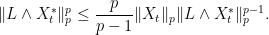
$\displaystyle \Vert L\wedge X^*_t\Vert_p^{p}\le\frac{p}{p-1}\Vert X_t\Vert_p\Vert L\wedge X^*_t\Vert_p^{p-1}.$

Finally, cancel ${\Vert L\wedge X^*_t\Vert_p^{p-1}}$ from both sides and take the limit ${L\uparrow\infty}$ to get the second inequality in the statement of the theorem.

Now, multiply both sides of (1) by ${K^{-1}}$ and integrating over a range ${[1,L]}$ for any ${L > 1}$ ,

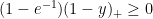
$\displaystyle \setlength\arraycolsep{2pt} \begin{array}{rcl} \displaystyle{\mathbb E}\left[(L\wedge X^*_t-1)_+\right] &\displaystyle=&\displaystyle {\mathbb E}\left[\int_1^L1_{\{X^*_t\ge K\}}\,dK\right]\smallskip\\ &\displaystyle=&\displaystyle \int_1^L{\mathbb P}(X^*_t\ge K)\,dK\smallskip\\ &\displaystyle\le &\displaystyle \int_1^LK^{-1}{\mathbb E}\left[1_{\{X^*_t\ge K\}}X_t\right]\,dK\smallskip\\ &\displaystyle=&\displaystyle {\mathbb E}\left[X_t\int_1^{1\vee(L\wedge X^*_t)}K^{-1}\,dK\right]\smallskip\\ &\displaystyle=&\displaystyle{\mathbb E}\left[X_t\log_+(L\wedge X^*_t)\right], \end{array}$

using the notation ${\log_+x\equiv\log(1\vee x)}$ . As we will show in a moment, the inequality

$\displaystyle x\log_+y+1\wedge y\le x\log x+e^{-1}y+1$

(2)

holds for nonnegative x and y. Adding ${{\mathbb E}[1\wedge X^*_t]}$ to both sides of the previous inequality and applying (2) with ${x=X_t}$ and ${y=L\wedge X^*_t}$ ,

$\displaystyle {\mathbb E}[L\wedge X^*_t]\le{\mathbb E}[X_t\log X_t+e^{-1}(L\wedge X^*_t)+1].$

Subtract ${e^{-1}{\mathbb E}[L\wedge X^*_t]}$ from both sides and take the limit ${L\uparrow\infty}$ to get the third inequality of the theorem.

It only remains to show that (2) holds for all nonnegative reals x and y. Moving all the terms to the same side, the inequality is equivalent to

$\displaystyle x\log x-x\log_+y+e^{-1}y+(1-y)_+\ge0.$

By differentiating with respect to x, the minimum of the left hand side occurs at ${x=e^{-1}(1\vee y)}$ , at which it takes the value ${(1-e^{-1})(1-y)_+\ge0}$ , proving (2) ⬜

5 thoughts on “Martingale Inequalities”

Mike says:

15 February 12 at 12:12 PM

This article was really helpful, thx.

PS: in the last line the constant p/(p-1) is missing…

1. George Lowther says:
  
  22 February 12 at 1:00 AM
  
  Fixed. Thanks.
  
Anonymous says:

1 March 12 at 11:06 AM

Hi George,

Just a small comment:
I think one needs to first consider a finite time grid to be able to assume that {X_t^* >= K} = {\tau <= t} (second line in proof of theorem 2) and the use MCT to get the result for countable time and continuous time in the cadlag case, like you mentioned in the planetmath proof.

Best,
Tigran

1. George Lowther says:
  
  1 March 12 at 11:50 PM
  
  Hi. You can do it that way, but it is not necessary to start by restricting to the finite case. I already proved the Debut theorem and optional sampling for continuous-time cadlag processes. As we assume the process is cadlag, these can be applied directly to the continuous time case.
  
Pingback: a nice optional sampling problem | Aquazorcarson's Blog

	Tavin on Class (D) Processes
	George Lowther on Filtrations and Adapted P…
	faceet on Filtrations and Adapted P…
	George Lowther on Filtrations and Adapted P…
	facet on Filtrations and Adapted P…
	Zoltan on Class (D) Processes
	Zoltan on Class (D) Processes
	ARS on Stopping Times and the Debut…
	George Lowther on Upcrossings, Downcrossings, an…
	George Lowther on Stopping Times and the Debut…

Martingale Inequalities

Published by George Lowther

5 thoughts on “Martingale Inequalities”

Leave a Reply Cancel reply

Like this:

Related

Published by George Lowther

5 thoughts on “Martingale Inequalities”

Leave a Reply Cancel reply