Spitzer’s formula is a remarkable result giving the precise joint distribution of the maximum and terminal value of a random walk in terms of the marginal distributions of the process. I have already covered the use of the reflection principle to describe the maximum of Brownian motion, and the same technique can be used for simple symmetric random walks which have a step size of ±1. What is remarkable about Spitzer’s formula is that it applies to random walks with any step distribution.
We consider partial sums
for an independent identically distributed (IID) sequence of real-valued random variables X1, X2, …. This ranges over index n = 0, 1, … starting at S0 = 0 and has running maximum
Spitzer’s theorem is typically stated in terms of characteristic functions, giving the distributions of (Rn, Sn) in terms of the distributions of the positive and negative parts, Sn+ and Sn–, of the random walk.
Theorem 1 (Spitzer) For α, β ∈ ℝ,
(1)
where ϕn, wn are the characteristic functions
As characteristic functions are bounded by 1, the infinite sums in (1) converge for |t|< 1. However, convergence is not really necessary to interpret this formula, since both sides can be considered as formal power series in indeterminate t, with equality meaning that coefficients of powers of t are equated. Comparing powers of t gives
(2)
and so on.
Spitzer’s theorem in the form above describes the joint distribution of the nonnegative random variables (Rn, Rn - Sn) in terms of the nonnegative variables (Sn+, Sn–). While this does have a nice symmetry, it is often more convenient to look at the distribution of (Rn, Sn) in terms of (Sn+, Sn), which is achieved by replacing α with α + β and β with –β in (1). This gives a slightly different, but equivalent, version of the theorem.
Theorem 2 (Spitzer) For α, β ∈ ℝ,
(3)
where ϕ̃n, w̃n are the characteristic functions
Taking β = 0 in either (1) or (3) gives the distribution of Rn in terms of Sn+,
(4)
I will give a proof of Spitzer’s theorem below. First, though, let’s look at some consequences, starting with the following strikingly simple result for the expected maximum of a random walk.
Corollary 3 For each n ≥ 0,
(5)
Proof: As Rn ≥ S1+ = X1+, if Xk+ have infinite mean then both sides of (5) are infinite. On the other hand, if Xk+ have finite mean then so do Sn+ and Rn. Using the fact that the derivative of the characteristic function of an integrable random variable at 0 is just i times its expected value, compute the derivative of (4) at α = 0,
Equating powers of t gives the result. ⬜
The expression for the distribution of Rn in terms of Sn+ might not be entirely intuitive at first glance. Sure, it describes the characteristic functions and, hence, determines the distribution. However, we can describe it more explicitly. As suggested by the evaluation of the first few terms in (2), each ϕn is a convex combination of products of the wn. As is well known, the characteristic function of the sum of random variables is equal to the product of their characteristic functions. Also, if we select a random variable at random from a finite set, then its characteristic function is a convex combination of those of the individual variables with coefficients corresponding to the probabilities in the random choice. So, (3) expresses the distribution of (Rn, Sn) as a random choice of sums of independent copies of (Sk+, Sk).
In fact, expressions such as (1,3) are common in many branches of maths, such as zeta functions associated with curves over finite fields. We have a power series which can be expressed in two different ways,
The left hand side is the generating function of the sequence an. The right hand side is a kind of zeta function associated with the sequence bn, and is sometimes referred to as the combinatorial zeta function. The logarithmic derivative gives Σnbntn-1, which is the generating function of bn+1. Continue reading “Spitzer’s Formula”→
In this post I look at the integral Xt = ∫0t 1{W≥0}dW for standard Brownian motion W. This is a particularly interesting example of stochastic integration with connections to local times, option pricing and hedging, and demonstrates behaviour not seen for deterministic integrals that can seem counter-intuitive. For a start, Xis a martingale so has zero expectation. To some it might, at first, seem that X is nonnegative and — furthermore — equals W ∨ 0. However, this has positive expectation contradicting the first property. In fact, X can go negative and we can compute its distribution. In a Twitter post, Oswin So asked about this very point, showing some plots demonstrating the behaviour of the integral.
Figure 1: Numerically evaluating ∫10 1{W≥0}dW
We can evaluate the integral as Xt = Wt ∨ 0 – 12Lt0 where Lt0 is the local time of W at 0. The local time is a continuous increasing process starting from 0, and only increases at times where W = 0. That is, it is constant over intervals on which W is nonzero. The first term, Wt ∨ 0 has probability density p(x) equal to that of a normal density over x > 0 and has a delta function at zero. Subtracting the nonnegative value L0t spreads out the density of this delta function to the left, leading to the odd looking density computed numerically in So’s Twitter post, with a peak just to the left of the origin and dropping instantly to a smaller value on the right. We will compute an exact form for this probability density but, first, let’s look at an intuitive interpretation in the language of option pricing.
Consider a financial asset such as a stock, whose spot price at time t is St. We suppose that the price is defined at all times t ≥ 0 and has continuous sample paths. Furthermore, suppose that we can buy and sell at spot any time with no transaction costs. A call option of strike price K and maturity T pays out the cash value (ST - K)+ at time T. For simplicity, assume that this is ‘out of the money’ at the initial time, meaning that S0 ≤ K.
The idea of option hedging is, starting with an initial investment, to trade in the stock in such a way that at maturity T, the value of our trading portfolio is equal to (ST - K)+. This synthetically replicates the option. A naive suggestion which is sometimes considered is to hold one unit of stock at all times t for which St ≥ K and zero units at all other times.The profit from such a strategy is given by the integral XT = ∫0T 1{S≥K}dS. If the stock only equals the strike price at finitely many times then this works. If it first hits K at time s and does not drop back below it on interval (s, t) then the profit at t is equal to the amount St – K that it has gone up since we purchased it. If it drops back below the strike then we sell at K for zero profit or loss, and this repeats for subsequent times that it exceeds K. So, at time T, we hold one unit of stock if its value is above K for a profit of ST – K and zero units for zero profit otherwise. This replicates the option payoff.
The idea described works if ST hits the strike K at a finite set of times,and also if the path of St has finite variation, in which case Lebesgue-Stieltjes integration gives XT = (ST - K)+. It cannot work for stock prices though! If it did, then we have a trading strategy which is guaranteed to never lose money but generates profits on the positive probability event that ST > K. This is arbitrage, generating money with zero risk, which should be impossible.
What goes wrong? First, Brownian motion does not have sample paths with finite variation and will not hit a level finitely often. Instead, if it reaches K then it hits the level uncountably often. As our simple trading strategy would involve buying and selling infinitely often, it is not so easy. Instead, we can approximate by a discrete-time strategy and take the limit. Choosing a finite sequence of times 0 = t0 < t1 < ⋯< tn = T, the discrete approximation is to hold one unit of the asset over the interval (ti, ti+1] if Sti ≥ K and zero units otherwise.
The discrete strategy involves buying one unit of the asset whenever its price reaches K at one of the discrete times and selling whenever it drops back below. This replicates the option payoff, except for the fact then when we buy above K we effectively overpay by amount Sti – K and, when we sell below K, we lose K – Sti. This results in some slippage from not being able to execute at the exact level,
So, our simple trading strategy generates profit (ST - K)+ – AT, missing the option value by amount AT. In the limit as n goes to infinity with time step size going to zero, the slippage AT does not go to zero. For equally spaced times, It can be shown that the number of times that spot crosses K is of order √n, and each of these times generates slippage of order 1/√n on average. So, in the limit, AT does not vanish and, instead, converges on a positive value equal to half the local time LTK.
Figure 2: Naive option hedge with slippage
Figure 2 shows the situation, with the slippage A shown on the same plot (using K as the zero axis, so they are on the same scale). We can just take K = 0 for an asset whose spot price can be positive or negative. Then, with S = W, our integral XT = ∫0T 1{W≥0}dW is the same as the payoff from the naive option hedge, or (ST)+ minus slippage L0T/2.
Now lets turn to a computation of the probability density of XT = WT ∨ 0 – LT0/2. By the scaling property of Brownian motion, the distribution of XT/√T does not depend on T, so we take T = 1 without loss of generality. The first trick to this is to make use of the fact that, if Mt = sups≤tWs is the running maximum then (|Wt|, Lt0)has the same joint distribution as (Mt - Wt, Mt). This immediately tells us that L10 has the same distribution as M1 which, by the reflection principle, has the same distribution as |W1|. Using
for the standard normal density, this shows that the local time L10 has probability density 2φ(x) over x > 0.
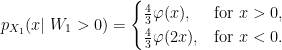
Next, as flipping the sign W does not impact either |W1| or L10, sgn(W1) is independent of these. On the event W1 < 0 we have X1 = –L10/2 which has density 4φ(2x) over x < 0. On the event W1 > 0, we have X1 = |W1|-L10/2, which has the same distribution as M1/2 – W1.
To complete the computation of the probability density of X1, we need to know the joint distribution of M1 and W1, which can be done as described in the post on the reflection principle. The probability that W1 is in an interval of width δx about a point x and that M1 > y, for some y > x is, by reflection, equal to the probability that W1 is in an interval of width δx about the point 2y – x. This has probability φ(2y - x)δx and, by differentiating in y, gives a joint probability density of 2φ′(x - 2y) for (W1, M1).
The expectation of f(X1) for bounded measurable function f can be computed by integrating over this joint probability density.
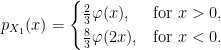
The substitution z = y/2 – x was applied in the inner integral, and the order of integration switched. The probability density of X1 conditioned on W1 > 0 is therefore,
Conditioned on W1 < 0, we have already shown that the density is 4φ(2x) over x < 0 so, taking the average of these, we obtain
This is plotted in figure 3 below, agreeing with So’s numerical estimation from the Twitter post shown in figure 1 above.
In a 1986 article of The American Mathematical Monthly written by Richard Guy, the following question was asked, and attributed to Bogusłav Tomaszewski: Consider n real numbers a1, …, an such that Σiai2 = 1. Of the 2n expressions |±a1±⋯±an|,
can there be more with value > 1 than with value ≤ 1?
A cursory attempt to find such real numbers ai where more of the absolute signed sums have value > 1 than have value ≤ 1 should be enough to convince you that it is, in fact, impossible. The answer was therefore expected to be no, it is not possible. This has claim since been known as Tomaszewski’s conjecture, and there have been many proofs of weaker versions over the years until, finally, in 2020, it was proved by Keller and Klein in the paper Proof of Tomaszewski’s Conjecture on Randomly Signed Sums.
where X1, …, Xn are independent ‘random signs’. That is, they have the Rademacher distribution ℙ(Xi = 1) = ℙ(Xi = -1) = 1/2. Then, Z has variance Σiai2 and each of the 2n values ±a1±⋯±an occurs with equal probability. So, Tomaszewski’s conjecture is the statement that
(2)
for unit variance Rademacher sums Z. It is usually stated in the equivalent, but more convenient form
(3)
I will discuss Tomaszewski’s conjecture and the ideas central to the proof given by Keller and Klein. I will not give a full derivation here. That would get very tedious, as evidenced both by the length of the quoted paper and by its use of computer assistance. However, I will prove the ‘difficult’ cases, which makes use of the tricks essential to Keller and Klein’s proof, with all remaining cases being, in theory, provable by brute force. In particular, I give a reformulation of the inductive stopping time argument that they used. This is a very ingenious trick that was introduced by Keller and Klein, and describing this is one of the main motivations for this post. Another technique also used in the proof is based on the reflection principle, in addition to some tricks discussed in the earlier post on Rademacher concentration inequalities.
To get a feel for Rademacher sums, some simple examples are shown in figure 1. I use the notation a = (a1, …, an) to represent the sequence with first n terms given by ai, and any remaining terms equal to zero. The plots show the successive partial sums for each sequence of values of the random signs (X1, X2, …), with the dashed lines marking the ±1 levels.
Figure 1: Example Rademacher sums
The examples demonstrate that ℙ(|Z| ≤ 1) can achieve the bound of 1/2 in some cases, and be strictly more in others. The top-left and bottom-right plots show that, for certain coefficients, |Z| has a positive probability of being exactly equal to 1 and, furthermore, the claimed bound fails for ℙ(|Z|< 1). So, the inequality is optimal in a couple of ways. These examples concern a small number of nonzero coefficients. In the other extreme, for a large number of small coefficients, the central limit theorem says that Z is approximately a standard normal and ℙ(|Z| ≤ 1) is close to Φ(1) – Φ(-1) ≈ 0.68. Continue reading “Tomaszewski’s Conjecture”→
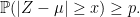
Concentration inequalities place lower bounds on the probability of a random variable being close to a given value. Typically, they will state something along the lines that a variable Z is within a distance x of value μ with probability at least p,
(1)
Although such statements can be made in more general topological spaces, I only consider real valued random variables here. Clearly, (1) is the same as saying that Z is greater than distance x from μ with probability no more than q = 1 – p. We can express concentration inequalities either way round, depending on what is convenient. Also, the inequality signs in expressions such as (1) may or may not be strict. A very simple example is Markov’s inequality,
In the other direction, we also encounter anti-concentration inequalities, which place lower bounds on on the probability of a random variable being at least some distance from a specified value, so take the form
While the examples given above of the Markov and Paley-Zygmund inequalities are very general, applying whenever the required moments exist, they are also rather weak. For restricted classes of random variables much stronger bounds can often be obtained. Here, I will be concerned with optimal concentration and anti-concentration bounds for Rademacher sums. Recall that these are of the form
for IID random variables X = (X1, X2, …) with the Rademacher distribution, ℙ(Xn = 1) = ℙ(Xn = -1) = 1/2, and a = (a1, a2, …) is a square-summable sequence. This sum converges to a limit with zero mean and variance
I discussed such sums at length in the posts on Rademacher series and the Khintchine inequality, and have been planning on making this follow-up post ever since. In fact, the L0 Khintchine inequality was effectively the same thing as an anti-concentration bound. It was far from optimal as presented there, and relied on the rather inefficient Paley-Zygmund inequality for the proof. Recently, though, a paper was posted on arXiv claiming to confirm conjectured optimal anti-concentration bounds which I had previous mentioned on mathoverflow. See Tight lower bounds for anti-concentration of Rademacher sums and Tomaszewski’s counterpart problem by Lawrence Hollom and Julien Portier.
While the form of the tight Rademacher concentration and anti-concentration bounds may seem surprising at first, being piecewise constant and jumping between rather arbitrary looking rational values at seemingly arbitrary points, I will explain why this is so. It is actually rather interesting and has been a source of conjectures over the past few decades, some of which have now been proved and some which remain open. Actually, as I will explain, many tight bounds can be proven in principle by direct computation, although it would be rather numerically intensive to perform in practice. In fact, some recent results — including those of Hollom and Portier mentioned above — were solved with the aid of a computer to perform the numerical legwork.
Anti-Concentration Bounds
Figure 1: Optimal anti-concentration bounds
For a Rademacher sum Z of unit variance, recall from the post on the Khintchine inequality that the anti-concentration bound
(3)
holds for all non-negative x ≤ 1. This followed from Payley-Zygmund together with the simple Khintchine inequality 𝔼[Z2] ≤ 3. However, this is sub-optimal and is especially bad in the limit as x increases to 1 where the bound tends to zero whereas, as we will see, the optimal bound remains strictly positive.
In the other direction if, for positive integer n, we choose coefficients a ∈ ℓ2 with ak = 1/√n for k ≤ n and zero elsewhere then, by the central limit theorem, Z = a·X tends to a standard normal distribution. as n becomes large. Hence
where Φ is the cumulative normal distribution function. So, any anti-concentration bound must be no more than this.
The optimal anti-concentration bounds have been open conjectures for a while, but are now proved and described by theorem 1 below, as plotted in figure 1. They are given by a piecewise constant function and, as clear from the plot, lie strictly between the simple Paley-Zymund bound and Gaussian probabilities.
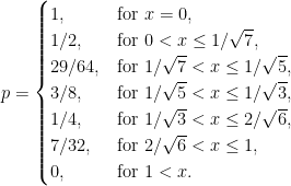
Theorem 1 The optimal lower bound p for the inequality ℙ(|Z| ≥ x) ≥ p for Rademacher sums Z of unit variance is,
At first sight, this result might seem a little strange. Why do the optimal bounds take this discrete set of values, and why does it jump at these arbitrary seeming values of x? To answer that, consider the distribution of a Rademacher sum. When all coefficients are small it approximates a standard normal and the anti-concentration probabilities approach those indicated by the ‘Gaussian bound’ in figure 1. However, these are not optimal, and the minimal probabilities are obtained at the opposite extreme with a small number n of relatively large coefficients and the remaining being zero. In this case, the distribution is finite with probabilities being multiples of 2–n, and the bound jumps when x passes through the discrete levels.
The values of a ∈ ℓ2 for which the stated bounds are achieved are not hard to find. For convenience, I use (a1, a2, …, an) to represent the sequence starting with the stated values and remaining terms being zero, ak = 0 for k > n. Also, if c is a numeral than ck will denote repeating this value k times.
Lemma 2 The optimal lower bound stated by theorem 1 for Rademacher sum Z = a·X is achieved with
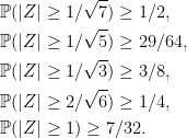
This is straightforward to verify by simply counting the number of sign values of (X1, |, Xn) for which |a·X| ≥ x and multiplying by 2–n. It does however show that it is impossible to do better than theorem 1 so that, if the bounds hold, they must be optimal. Also, as ℙ(|Z| ≥ x) is decreasing in x, to establish the result it is sufficient to show that the bounds hold at the values of x where it jumps. This reduces theorem 1 to the following finite set of inequalities.
Theorem 3 A Rademacher sum Z of unit variance satisfies,
The last of these has been an open conjecture for years since it was mentioned in a 1996 paper by Oleszkiewicz. I asked about the first one in a 2021 mathoverflow question, and also mentioned the finite set of values x at which the optimal bound jumps, hinting at the full set of inequalities, which was the desired goal. Finally, in 2023, a preprint appeared on arXiv claiming to prove all of these. While I have not completely verified the proof and the computer programs used myself, it does look likely to be correct.
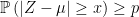
Although the bounds given above are all for anti-concentration about 0, a simple trick shows that they will also hold about any real value.
Lemma 4 Suppose that the inequality ℙ(|Z| ≥ x) ≥ p holds for all Rademacher sums Z of unit variance. Then the anti-concentration bound
also holds about every value μ.
Proof: If Z = a·X and, independently, Y is a Rademacher random variable, then Z + μY is a Rademacher sum of variance 1 + μ2. This follows from the fact that it has the same distribution as b·X where b = (μ, a1, a2, …). So,
By symmetry of the distribution of Z, both probabilities on the right are equal giving,
implying the result. ⬜
You have probably noted already, that all of the coefficients described in lemma 2 are of the form (1n)/√n. That is, they are a finite a sequence of equal values with the remaining terms being zero. In fact, it has been conjectured that all optimal concentration and anti-concentration bounds (about 0) for Rademacher sums can be attained in this way. This is attributed to Edelman dating back to private communications in 1991. If true, it would turn the process of finding and proving such optimal bounds into a straightforward calculation but, unfortunately, in 2012, the conjecture was shown to be false by Pinelis for some concentration inequalities.
Before moving on, let’s mention how such bounds can be discovered in the first place. Running a computer simulation for randomly chosen finite sequences of coefficients very quickly converges on the optimal values. As soon as we randomly select values close to those given by lemma 2, we obtain the exact bounds and any further simulations only serve to verify that these hold. Running additional simulations with coefficients chosen randomly in the neighbourhood of points where the bound is attained, and near certain ‘critical’ values where the bound looks close to being broken, further strengthens the belief that they are indeed optimal. At least, this is how I originally found them before asking the mathoverflow question, although this is still far from a proof.
Probability and measure theory relies on the concept of measurable sets. On the real numbers ℝ, in particular, there are several different sigma-algebras which are commonly used, and a set is said to be measurable if it lies in the one under consideration. Probabilities and measures are only defined for events lying in a specific sigma-algebra, so it is essential to know if sets are measurable. Fortunately, most simply constructed events will indeed be measurable, but this is not always the case. In fact, once we start working with more complex setups, such as continuous-time stochastic processes observed at random times, non-measurable sets occur more commonly than might be expected. To avoid such issues, it is usual to enlarge the underlying sigma-algebra defining a probability space as much as possible.
The Borel sets form the smallest sigma-algebra containing the open sets or, equivalently, containing all intervals. This is denoted as , which I will also shorten to . An explicit construction of a non-Borel set was given by Lusin in 1927. Every irrational real number can be expressed uniquely as a continued fraction
where a0 is an integer and ai are positive integers for i ≥ 1. Lusin considered the set of irrationals whose continued fraction coefficients contain a subsequence ak1, ak2, … such that each term is a divisor of the subsequent term.
Other examples can be given along similar lines to Lusin’s. Every real number has a binary expansion
where a0 is an integer and ai is in {0, 1} for each i ≥ 1. Consider the set of reals having a binary expansion for which there is an infinite sequence of positive integers k1, k2, …, each term strictly dividing the next, such that aki = 1. I will give proofs that these examples are non-Borel in this post.
There is a general method of enlarging sigma-algebras known as the completion. Consider a measure μ defined on a measurable space consisting of sigma-algebra on set X. The completion consists of all subsets S ⊆ X which can be sandwiched between sets in whose difference has zero measure. That is, A ⊆ S ⊆ B for with μ(B ∖ A) = 0. It can be shown that is a sigma-algebra containing , and μ uniquely extends to a measure on this by taking μ(S) = μ(A) = μ(B) for S, A, B as above.
The Lebesgue measure λ is uniquely defined on the Borel sets by specifiying its value on intervals as λ((a, b)) = b – a. The completion is the Lebesgue sigma-algebra, which I will denote by . Usually, when saying that a subset of the reals is measurable without further qualification, it is understood to mean that it is in . The non-Borel set constructed by Lusin can be shown to be measurable (in fact, its complement has zero Lebesgue measure).
While the Lebesgue measure extends uniquely to , this is not true for for all measures defined on the Borel sigma-algebra. In particular, it will not be true for singular measures, which assign a positive value to some Lebesgue-null sets. An example is the uniform probability measure (or, Haar measure) on the Cantor middle-thirds setC. This has zero Lebesgue measure, so every subset of C is in , but the uniform measure on C cannot be extended uniquely to all subsets. For this reason, universal completions are often used. For a measurable space , the universal completion consists of the subsets of X which lie in the completion of with respect to every possible sigma-finite measure.
The intersection is taken over all sigma-finite measures μ on . It is enough to take the intersection over finite or, even, probability measures, since every sigma-finite measure is equivalent to such. The universal completion is a bit tricky to understand in an explicit way but, by construction, all sigma-finite measures on a sigma-algebra extend uniquely to its universal completion. It can be shown that Lusin’s example of a non-Borel set does lie in the universal completion .
Finally, the power set consisting of all subsets of a set X is a sigma-algebra. For uncountable sets such as the reals, this is often too large to be of use and measures cannot be extended in any unique way. However, we have four common sigma-algebras of the real numbers,
(1)
In this post, I show that each of these inclusions is strict. That is, there are subsets of the reals which are not Lebesgue measurable, there are Lebesgue sets which are not in the universal completion , and there are sets in which are not Borel. Lusin’s construction is an example of the latter. The strictness of the other two inclusions does depend crucially on the axiom of choice so, unlike Lusin’s set, the examples demonstrating that these are strict are not explicit. Continue reading “Non-Measurable Sets”→
I continue the investigation of discrete barrier approximations started in an earlier post. The idea is to find good approximations to a continuous barrier condition, while only sampling the process at a discrete set of times. The difference now is that I will look at model independent methods which do not explicitly depend on properties of the underlying process, such as the volatility. This will enable much more generic adjustments which can be applied more easily and more widely. I point out now, the techniques that I will describe here are original research and cannot currently be found in the literature outside of this blog, to the best of my knowledge.
Recall that the problem is to compute the expected value of a function of a stochastic process X,
(1)
which depends on whether or not the process crosses a continuous barrier level K. In many applications, such as with Monte Carlo simulation, we typically only sample X at a discrete set of times 0 < t1 < t2 < ⋯< tn = T. In that case, the continuous barrier is necessarily approximated by a discrete one
(2)
As we saw, this converges slowly as the number n of sampling times increases, with the error between this and the limiting continuous barrier (1) only going to zero at rate 1/√n.
A barrier adjustment as described in the earlier post is able to improve this convergence rate. If X is a Brownian motion with constant drift μ and positive volatility σ, then the discrete barrier level K is shifted down by an amount βσ√δt where β ≈ 0.5826 is a constant and δt = T/n is the sampling width. We are assuming, for now, that the sampling times are equally spaced. As was seen, using the shifted barrier level in (2) improves the rate of convergence. Although we did not theoretically derive the new convergence rate, numerical experiment suggests that it is close to 1/n.
Another way to express this is to shift the values of X up,
(3)
Then, (2) is replaced to use these shifted values, which are a proxy for the maximum value of X across each of the intervals (ti-1, ti),
(4)
As it is equivalent to shifting the level K down, we still obtain the improved rate of convergence.
This idea is especially useful because of its generality. For non-equally spaced sampling times, the adjustment (3) can still be applied. Now, we just set δt = ti – ti-1 to be the spacing for the specific time, so depends on index i. It can also be used for much more general expressions than (1). Any function of X which depends on whether or not it crosses a continuous barrier can potentially make use of the adjustment described. Even if X is an Ito process with time dependent drift and volatility
(5)
the method can be applied. Now, the volatility in (3) is replaced by an average value across the interval (ti-1, ti).
The methods above are very useful, but there is a further improvement that can be made. Ideally, we would not have to specify an explicit value of the volatility σ. That is, it should be model independent. There are many reasons why this is desirable. Suppose that we are running a Monte Carlo simulation and generate samples of X at the times ti. If the simulation only outputs values of X, then this is not sufficient to compute (3). So, it will be necessary to update the program running the simulation to also output the volatility. In some situations this might not be easy. For example, X could be a complicated function of various other processes and, although we could use Ito’s lemma to compute the volatility of X from the other processes, it could be messy. In some situations we might not even have access to the volatility or any method of computing it. For example, the values of X could be computed from historical data. We could be looking at the probability of stock prices crossing a level by looking at historical close fixings, without access to the complete intra-day data. In any case, a model independent discrete barrier adjustment would make applying it much easier.
Removing Volatility Dependence
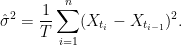
How can the volatility term be removed from adjustment (3)? One idea is to replace it by an estimator computed from the samples of X, such as
While this would work, at least for a constant volatility process, it does not meet the requirements. For a general Ito process (5) with stochastic volatility, using an estimator computed over the whole time interval [0, T] may not be a good approximation for the volatility at the time that the barrier is hit. A possible way around this is for the adjustment (3) applied at time ti to only depend on a volatility estimator computed from samples near the time. This would be possible, although it is not clear what is the best way to select these times. Besides, an important point to note is that we do not need a good estimate of the volatility, since that is not the goal here.
As explained in the previous post, adjustment (3) works because it corrects for the expected overshoot when the barrier is hit. Specifically, at the first time for which Mi ≥ K, the overshoot is R = Xti – K. If there was no adjustment then the overshoot is positive and the leading order term in the discrete barrier approximation error is proportional to 𝔼[R]. The positive shift added to Xti is chosen to compensate for this, giving zero expected overshoot to leading order, and reducing the barrier approximation error. The same applies to any similar adjustment. As long as there is sufficient freedom in choosing Mi, then it should be possible to do it in a way that has zero expected overshoot. Taking this to the extreme, it should be possible to compute the adjustment at time ti using only the sampled values Xti-1 and Xti.
Figure 1: Barrier overshoot
Consider adjustments of the form
for θ: ℝ2 → ℝ. By model independence, if this adjustment applies to a process X, then it should equally apply to the shifted and scaled processes X + a and bX for constants a and b > 0. Equivalently, θ satisfies the scaling and translation invariance,
(6)
This restricts the possible forms that θ can take.
Lemma 1 A function θ: ℝ2 → ℝ satisfies (6) if and only if
for constants p, c.
Proof: Write θ(0, u) as the sum of its antisymmetric and symmetric parts
By scaling invariance, the first term on the right is proportional to u and the second is proportional to |u|. Hence,
for constants p and c. Using translation invariance,
as required. ⬜
I will therefore only consider adjustments where the maximum of the process across the interval (ti-1, ti) is replaced by
(7)
According to (3), the barrier condition supt≤TXt ≥ K is replaced by the discrete approximation maxiMi ≥ K.
There are various ways in which (7) can be parameterized, but this form is quite intuitive. The term pXti + (1 - p)Xti-1 is an interpolation of the path of X, and c|Xti – Xti-1| represents a shift proportional to the sample deviation across the interval replacing the σ√δt term of the simple shift (3). The purpose of this post is to find values for p and c giving a good adjustment, improving convergence of the discrete approximation.
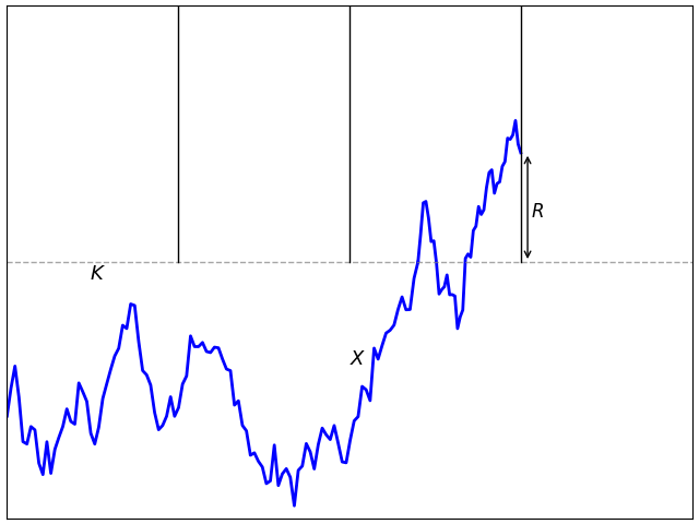
Figure 2: Adjusted barrier overshoot
The discrete barrier condition Mi ≥ K given by (7) can be satisfied while the process is below the barrier level, giving a negative barrier ‘overshoot’ R = Xti – K as in figure 2. As we will see, this is vital to obtaining an accurate approximation for the hitting probability. Continue reading “Model-Independent Discrete Barrier Adjustments”→
It is quite common to consider functions of real-time stochastic process which depend on whether or not it crosses a specified barrier level K. This can involve computing expectations involving a real-valued process X of the form
(1)
for a positive time T and function f: ℝ → ℝ. I am using the notation 𝔼[A;S] to denote the expectation of random variable A restricted to event S, or 𝔼[A1S].
One example is computing prices of financial derivatives such as barrier options, where T represents the expiration time and f is the payoff at expiry conditional on hitting upper barrier level K. A knock-in call option would have the final payoff f(x) = (x - a)+ for a contractual strike of a. Knock-out options are similar, except that the payoff is conditioned on not hitting the barrier level. As the sum of knock-in and knock-out options is just an option with no barrier, both cases involve similar calculations.
Alternatively, the barrier can be discrete, meaning that it only involves sampling the process at a finite set of times 0 ≤ t1 ≤ ⋯ ≤ tn ≤ T. Then, equation (1) is replaced by
(2)
Naturally, sampling at a finite set of times will reduce the probability of the barrier being reached and, so, if f is nonnegative then (2) will have a lower value than (1). It should still converge though as n goes to infinity and the sampling times become dense in the interval.
If the underlying process X is Brownian motion or geometric Brownian motion, possibly with a constant drift, then there are exact expressions for computing (1) in terms of integrating f against a normal density. See the post on the reflection principle for more information. However, it is difficult to find exact expressions for the discrete barrier (2) other than integrating over high-dimensional joint normal distributions. So, it can be useful to approximate a discrete barrier with analytic formulas for the continuous barrier. This is the idea used in the classic 1997 paper A Continuity Correction for Discrete Barrier Options by Broadie, Glasserman and Kou (freely available here).
We may want to compute the continuous barrier expectation (1) using Monte Carlo simulation. This is a common method, but involves generating sample paths of the process X at a finite set of times. This means that we are only able to sample at these times so, necessarily, are restricted to discrete barrier calculations as in (2).
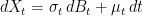
I am primarily concerned with the second idea This is a very general issue, since Monte Carlo simulation is a common technique used in many applications. However, as it only represents sample paths at discrete time points, it necessarily involves discretely approximating continuous barrier levels. You may well ask why we would even want to use Monte Carlo if, as I mentioned above, there are exact expressions in these cases.In answer, such formulas only hold in very restrictive situations where the process X is a Brownian motion or geometric Brownian motion with constant drift. More generally it could be an ‘Ito process’ of the form
(3)
where B is standard Brownian motion. This describes X as a stochastic integral with respect to the predictable integrands σ and μ, which represent the volatility and drift of the process. Strictly speaking, these are ‘linear’ volatility and drift terms, rather than log-linear as used in many financial models applied to nonnegative processes such as stock prices. This is simply the choice made here, since this post is addressing a general mathematical problem of approximating continuous barriers and not restricting to such specific applications.
If the volatility and drift terms in (3) are not constant, then the exact formulas no longer hold. This is true, even if they are deterministic functions of time. In practice, these terms are often stochastic and can be rather general, in which case trying to find exact expressions is an almost hopeless task. Even though I concentrate on the case with constant volatility and drift in any calculations performed here, this is for convenience of exposition. The idea is that, as long as σ is piecewise continuous then, locally, it is well approximate as constant and the techniques discussed here should still apply.
In addition to considering general Ito processes (3), the ideas described here will apply to much more general functions of the process X than stated in (1). In the financial context, this means more general payoffs than simple knock-in or knock-out options. For example, autocallable trades involve a down-and-in put option but, additionally, contain a discrete set of upper barriers which cause the trade to make a final payment and terminate. They may also allow the issuer to early terminate the trade on a discrete set of dates. Furthermore, trades can depend on different assets with separate barriers on each of them, or on the average of a basket of assets, or have different barrier levels in different time periods. The list of possibilities is endless but, the idea is that each continuous barrier inside a complex payoff will be approximated by discretely sampled barrier conditions.
For efficiency, we may also want to approximate a discrete barrier with a large number of sampling times by one with fewer. The methods outlined in the post can also be used for this. In particular, the simple barrier shift described below could be used by taking the difference between the shift computed for the times actually sampled and the one for the required sample times. I do not go into details of this, but mention it now give an idea of the generality of the technique.
Figure 1: Discrete barrier approximation error
Let’s consider simply approximating a continuous barrier in (1) by the discrete barrier in (2). This will converge as the number of sampling times ti increases but, the problem is, it converges very slowly. We can get an idea of the order of the error when the sampling times have a δt spacing which, with equally spaced times, is given by δt = T/n. This is as shown in figure 1 above. When the process first hits the continuous barrier level, it will be on average about δt/2 before the next sampling time. If X behaves approximately like a Brownian motion with volatiity σ over this interval then it will have about 50% chance of being above K at the next discrete time. On the other hand, it will be below K with about 50% probability, in which case with will drop a distance proportional to σ√δt below on average. This means that if the continuous barrier is hit, there is a probability roughly proportional to σ√δt that the discrete barrier is not hit. So, the error in approximating a continuous barrier (1) by the discrete case (2) is of the order of σ√δt which only tends to zero at rate 1/√n. Continue reading “Discrete Barrier Approximations”→
In stochastic calculus it is common to work with processes adapted to a filtered probability space. As with probability space extensions, It can sometimes be necessary to enlarge the underlying space to introduce additional events and processes. For example, many diffusions and local martingales can be expressed as an integral with respect to Brownian motion but, sometimes, it may be necessary to enlarge the space to make sure that it includes a Brownian motion to work with. Also, in the theory of stochastic differential equations, finding solutions can sometimes require enlarging the space.
Extending a probability space is a relatively straightforward concept, which I covered in an earlier post. Extending a filtered probability space is the same, except that it also involves enlarging the filtration . It is important to do this in a way which does not destroy properties of existing processes, such as their distributions conditional on the filtration at each time.
Let’s consider a filtered probability space . An enlargement
is, firstly, an extension of the probability spaces. It is a map from Ω′ to Ω measurable with respect to and , and preserving probabilities. So ℙ′(π-1E) = π(E) for all . In addition, it is required to be measurable for each time t ≥ 0, meaning that for all . Consequently, any adapted process Xt lifts to an adapted process X∗t = π∗Xt on the larger space, defined by X∗t(ω) = Xt(π(ω)).
As with extensions of probability spaces, this can be considered in two steps. First, we extend to the filtered probability space on Ω′ with induced sigma-algebra consisting of sets π-1E for , and to the filtration . This is essentially a no-op, since events and random variables on the original filtered probability space are in one-to-one correspondence with those on the enlarged space, up to zero probability events. Next, the sigma-algebras are enlarged to and . This is where new random events are added to the event space and filtration.
Such arbitrary extensions are too general for many uses in stochastic calculus where we merely want to add in some additional source of randomness. Consider, for example, a standard Brownian motion B defined on the original space so that, for any times s < t, Bt – Bs is normal and independent of . Does it necessarily lift to a Brownian motion on the enlarged space? The answer to this is no! It need not be the case that B∗t – B∗s is independent of . For an extreme case, consider the situation where and π is the identity, so there is no enlargement of the sample space. If the filtration is is extended to the maximum, , consider what happens to our Brownian motion. The increment Bt – Bs is -measurable, so is not independent of it. In fact, conditioned on , the entire path of B is deterministic. It is definitely not a Brownian motion with respect to this new filtration. Similarly, martingales, submartingales and supermartingales will not remain as such if we pass to this enlarged filtration.
The idea is that, if for random variables X, Y defined on our original probability space, then this relation should continue to hold in the extension. It is required that . This is exactly relative independence of and over .
According to Kolmogorov’s axioms, to define a probability space we start with a set Ω and an event space consisting of a sigma-algebra F on Ω. A probability measure ℙ on this gives the probability space (Ω, F , ℙ), on which we can define random variables as measurable maps from Ω to the reals or other measurable space.
However, it is common practice to suppress explicit mention of the underlying sample spaceΩ. The values of a random variable X: Ω → ℝ are simply written as X, rather than X(ω) for ω ∈ Ω. It is intuitively thought of as a real number which happens to be random, rather than a function. For one thing, we usually do not really care what the sample space is and, instead, only care about events and their probabilities, and about random variables and their expectations. This philosophy has some benefits. Frequently, when performing constructions, it can be useful to introduce new supplementary random variables to work with. It may be necessary to enlarge the sample space and add new events to the sigma-algebra to accommodate these. If the underlying space is not set in stone then this is straightforward to do, and we can continue to work with these new variables as if they were always there from the start.
Definition 1 An extension π of a probability space (Ω, F , ℙ) to a new space (Ω′, F ′, ℙ′),
is a probability preserving measurable map π: Ω′ → Ω. That is, ℙ′(π-1E) = ℙ(E) for events E ∈ F .
By construction, events E ∈ F pull back to events π-1E ∈ F ′ with the same probabilities. Random variables X defined on (Ω, F , ℙ) lift to variables π∗X with the same distribution defined on (Ω′, F ′, ℙ′), given by π∗X(ω) ≡ X(π(ω)). I will use the notation X∗ in place of π∗X for brevity although, in applications, it is common to reuse the same symbol X and simply note that we are now working with respect to an enlarged the probability space if necessary.
The extension can be thought of in two steps. First, the enlargement of the sample space, π: Ω′ → Ω on which we induce the sigma algebra π∗F consisting of events π-1E for E ∈ F , and the measure ℙ′(π-1E) = ℙ(E). This is essentially a no-op, since events and random variables on the initial space are in one-to-one correspondence with those on the enlarged space (at least, up to zero probability events). Next, we enlarge the sigma-algebra to F ′ ⊇ π∗F and extend the measure ℙ′ to this. It is this second step which introduces new events and random variables.
Since we may want to extend a probability space more than a single time, I look at how these combine. Consider an extension π of the original probability space, and then a further extension ρ of this.
These can be combined into a single extension ϕ = π○ρ of the original space,
Lemma 2 The composition ϕ = π○ρ is itself an extension of the probability space.
Proof: As compositions of measurable maps are measurable, it is sufficient to check that ϕ preserves probabilities. This is straightforward,
for all E ∈ F . ⬜
So far, so simple. The main purpose of this post, however, is to look at the situation with two separate extensions of the same underlying space. Both of these will add in some additional source of randomness, and we would like to combine them into a single extension.
Separate probability spaces can be combined by the product measure, which is the measure on the product space for which the projections onto the original spaces preserves probability, and for which the sigma-algebras generated by these projections are independent. Recall that a pair of sigma-algebras F and G defined on a probability space are independent if, for any sets A ∈ F and B ∈ G then ℙ(A ∩ B) = ℙ(A)ℙ(B).
Combining extensions of probability spaces will, instead, make use of relative independence.
Definition 3 Let (Ω, F , ℙ) be a probability space. Two sub-sigma-algebras G , H ⊆ F are relatively independent over a third sigma-algebra K ⊆ G ∩ H if
(1)
for all A ∈ G and B ∈ H .
It can be shown that the following properties are each equivalent to this definition;
𝔼[XY|K ] = 𝔼[X|K ]𝔼[Y|K ] for all bounded G -measurable random variables X and H -measurable Y.
𝔼[X|G ] = 𝔼[X|K ] for all bounded H -measurable X.
𝔼[X|H ] = 𝔼[X|K ] for all bounded G -measurable X.
Once a probability measure is specified separately on G and H then its extension to the sigma-algebra generated by G ∪ H , if it exists, is uniquely determined by relative independence. This is a consequence of the pi-system lemma, since (1) defines it on the events {A ∩ B: A ∈ G , B ∈ H }, which is a pi-system generating the same sigma-algebra.
Now consider two separate extensions π1 and π2 of the same underlying probability space,
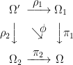
As maps between sets, these can both be embedded into a single extension known as the pullback or fiber product. This is the set Ω′= Ω1 ×Ω Ω2 defined by
Defining projection maps ρi: Ω′ → Ωi by
results in a commutative square with ϕ ≡ π1○ρ1 = π2○ρ2,
In fact, Ω′ is exactly the cartesian product Ω1 × Ω2 restricted to the subset on which π1○ρ1 and π2○ρ2 agree.
This constructs an extension ϕ of the sample space containing π1 and π2 as sub-extensions. However, it still needs to be made into a probability space. Use the smallest sigma-algebra F ′ on Ω′ making ρ1, ρ2 into measurable maps, which is generated by ρ1∗F 1 ∪ ρ2∗F 2. The probability measure ℙ′ on (Ω′, F ′) is uniquely determined on each of the sub-sigma-algebras by the requirement that ρi preserve probabilities,
for i = 1, 2 and A ∈ F i. These necessarily agree on ϕ∗F ⊆ ρ1∗F 1 ∩ ρ2∗F 2,
for A ∈ F . The natural way to extend ℙ′ to all of F ′ is to use relative independence over ϕ∗F .
Definition 4 The relative product of the extensions π1 and π2 is the extension
with ϕ, Ω′, F ′ constructed as above, and ℙ′ is the unique probability measure for which the projections ρ1, ρ2 preserve probabilities, and for which ρ1∗F 1 and ρ2∗F 2 are relatively independent over ϕ∗F .
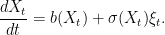
Stochastic differential equations (SDEs) form a large and very important part of the theory of stochastic calculus. Much like ordinary differential equations (ODEs), they describe the behaviour of a dynamical system over infinitesimal time increments, and their solutions show how the system evolves over time. The difference with SDEs is that they include a source of random noise., typically given by a Brownian motion. Since Brownian motion has many pathological properties, such as being everywhere nondifferentiable, classical differential techniques are not well equipped to handle such equations. Standard results regarding the existence and uniqueness of solutions to ODEs do not apply in the stochastic case, and cannot readily describe what it even means to solve such as system. I will make some posts explaining how the theory of stochastic calculus applies to systems described by an SDE.
Consider a stochastic differential equation describing the evolution of a real-valued process{Xt}t≥0,
(1)
which can be specified along with an initial condition X0 = x0. Here, b is the drift specifying how X moves on average across the dt time, σ is a volatility term giving the amplitude of the random noise and W is a driving Brownian motion providing the source of the randomness. There are numerous situations where equations such as (1) are used, with applications in physics, finance, filtering theory, and many other areas.
In the case where σ is zero, (1) is just an ordinary differential equation dX/dt = b(X). In the general case, we can informally think of dividing through by dt to give an ODE plus an additional noise term
(2)
I have set ξt = dWt/dt which can be thought of as a process whose values at each time are independent zero-mean random variables. As mentioned above, though, Brownian motion is not differentiable so this does not exist in the usual sense. While it can be described by a kind of random distribution, even distribution theory is not well-equipped to handle such equations involving multiplying by the nondifferentiable process σ(Xt). Instead, (1) can be integrated to obtain
(3)
where the right-hand-side is interpreted using stochastic integration with respect to the semimartingaleW. Likewise, X will be a semimartingale, and such solutions are often referred to as diffusions.
The differential form (1) can be interpreted as a shorthand for the integral expression (3), which I will do in these notes. It can be generalized to n-dimensional processes by allowing b to take values in ℝn, σ(x) to be an n × m matrix, and W to be an m-dimensional Brownian motion. That is, W = (W1, …, Wm) where Wi are independent Brownian motions. I will sometimes write this as
where the summation convention is being applied, with subscripts or superscripts occuring more than once in a single term being summed from 1 to n.
Unlike ODEs, when dealing with SDEs we need to consider what underlying probability space the solution is defined with respect to. This leads to the existence of different classes of solutions.
Strong solutions where X can be expressed as a measurable function of the Brownian motion W or, equivalently, X is adapted to its natural filtration.
Weak solutions where X need not be a function of W. Such cases may require additional randomness so may not exist on the probability space with respect to which the Brownian motion W is defined. It can be necessary to extend the filtered probability space to construct these solutions.
Likewise, when considering uniqueness of solutions, there are different ways this occurs.
Pathwise uniqueness where, up to indistinguishability, there is only one solution X. This should hold not just on one specific space containing a Brownian motion W, but on all such spaces. That is, weak solutions should be unique.
Uniqueness in law where there may be multiple pathwise solutions, but their distribution is uniquely determined by the SDE.
There are various general conditions under which strong solutions and pathwise uniqueness are guaranteed for SDE (1) , such as the Itô result for Lipschitz continuous coefficients. I covered this situation in a previous post.
Other than using the SDE (1), such systems can also be described by an associated differential operator. For the n-dimensional case set a(x) = σ(x)σ(x)T, which is an n × n positive semidefinite matrix. Then, the second order operator L can be defined
operating on twice continuously differentiable functions f: ℝn → ℝ. Being able to effortlessly switch between descriptions using the SDE (1) and the operator L is a huge benefit when working with such systems. There are several different ways in which the operator can be used to describe a stochastic process, all of which relate to weak solutions and uniqueness in law of the SDE.
Markov Generator: A Markov process is a weak solution to the SDE (1) if its infinitesimal generator is L. That is, if the transition function is Pt then,
for suitably regular functions f.
Backwards Equation: For a function f: ℝn × ℝ+ → ℝ, f(t, Xt) is a local martingale if and only if it solves the partial differential equation (PDE)
Consequently, for any time t > 0 and function g: ℝd → ℝ, if we let f be a solution to the PDE above with boundary condition f(x, t) = g(x) then, assuming integrability conditions, the conditional expectations at times s < t are
If the conditions are satisfied, this describes a Markov process and gives its transition probabilities, describing the distribution of X and implying uniqueness in law.
Forward Equation: Assuming that it is sufficiently smooth, the probability density p(t, x) of Xt satisfies the PDE
where LT is the transpose of operator L
If this PDE has a unique solution for given initial distribution, then this uniquely determines the distribution of Xt. So, if unique solutions to the forward equation exist starting at every future time, it gives uniqueness in law for X.
Martingale problem: Any weak solution to SDE (1) satisfies the property that
is a local martingale for twice continuously differentiable functions f: ℝn → ℝ. This approach, which was pioneered by Stroock and Varadhan, has many benefits over the other applications of operator L described above, since it applies much more generally. We do not need to a-priori impose any properties on X such as being Markov, and as the test functions f are chosen at will, they automatically satisfy the necessary regularity properties. As well as being a very general way to describe solutions to a stochastic dynamical system, it turns out to be very fruitful. The striking and far-reaching Stroock–Varadhan uniqueness theorem, in particular, guarantees existence and uniqueness in law so long as a is continuous and positive definite and b is locally bounded.


![\displaystyle \begin{aligned} \phi_n(\alpha,\beta)&={\mathbb E}\left[e^{i\alpha R_n+i\beta(R_n-S_n)}\right],\\ w_n(\alpha,\beta)&={\mathbb E}\left[e^{i\alpha S_n^++i\beta S_n^-}\right]\\ &={\mathbb E}\left[e^{i\alpha S_n^+}\right]+{\mathbb E}\left[e^{i\beta S_n^-}\right]-1. \end{aligned}](https://s0.wp.com/latex.php?latex=%5Cdisplaystyle+%5Cbegin%7Baligned%7D+%5Cphi_n%28%5Calpha%2C%5Cbeta%29%26%3D%7B%5Cmathbb+E%7D%5Cleft%5Be%5E%7Bi%5Calpha+R_n%2Bi%5Cbeta%28R_n-S_n%29%7D%5Cright%5D%2C%5C%5C+w_n%28%5Calpha%2C%5Cbeta%29%26%3D%7B%5Cmathbb+E%7D%5Cleft%5Be%5E%7Bi%5Calpha+S_n%5E%2B%2Bi%5Cbeta+S_n%5E-%7D%5Cright%5D%5C%5C+%26%3D%7B%5Cmathbb+E%7D%5Cleft%5Be%5E%7Bi%5Calpha+S_n%5E%2B%7D%5Cright%5D%2B%7B%5Cmathbb+E%7D%5Cleft%5Be%5E%7Bi%5Cbeta+S_n%5E-%7D%5Cright%5D-1.+%5Cend%7Baligned%7D+&bg=ffffff&fg=000000&s=0&c=20201002)

![\displaystyle \begin{aligned} \tilde\phi_n(\alpha,\beta)&={\mathbb E}\left[e^{i\alpha R_n+i\beta S_n}\right],\\ \tilde w_n(\alpha,\beta)&={\mathbb E}\left[e^{i\alpha S_n^++i\beta S_n}\right]. \end{aligned}](https://s0.wp.com/latex.php?latex=%5Cdisplaystyle+%5Cbegin%7Baligned%7D+%5Ctilde%5Cphi_n%28%5Calpha%2C%5Cbeta%29%26%3D%7B%5Cmathbb+E%7D%5Cleft%5Be%5E%7Bi%5Calpha+R_n%2Bi%5Cbeta+S_n%7D%5Cright%5D%2C%5C%5C+%5Ctilde+w_n%28%5Calpha%2C%5Cbeta%29%26%3D%7B%5Cmathbb+E%7D%5Cleft%5Be%5E%7Bi%5Calpha+S_n%5E%2B%2Bi%5Cbeta+S_n%7D%5Cright%5D.+%5Cend%7Baligned%7D+&bg=ffffff&fg=000000&s=0&c=20201002)
![\displaystyle \sum_{n=0}^\infty {\mathbb E}\left[e^{i\alpha R_n}\right]t^n=\exp\left(\sum_{n=1}^\infty {\mathbb E}\left[e^{i\alpha S_n^+}\right]\frac{t^n}n\right)](https://s0.wp.com/latex.php?latex=%5Cdisplaystyle+%5Csum_%7Bn%3D0%7D%5E%5Cinfty+%7B%5Cmathbb+E%7D%5Cleft%5Be%5E%7Bi%5Calpha+R_n%7D%5Cright%5Dt%5En%3D%5Cexp%5Cleft%28%5Csum_%7Bn%3D1%7D%5E%5Cinfty+%7B%5Cmathbb+E%7D%5Cleft%5Be%5E%7Bi%5Calpha+S_n%5E%2B%7D%5Cright%5D%5Cfrac%7Bt%5En%7Dn%5Cright%29+&bg=ffffff&fg=000000&s=0&c=20201002)
![\displaystyle {\mathbb E}[R_n]=\sum_{k=1}^n\frac1k{\mathbb E}[S_k^+].](https://s0.wp.com/latex.php?latex=%5Cdisplaystyle+%7B%5Cmathbb+E%7D%5BR_n%5D%3D%5Csum_%7Bk%3D1%7D%5En%5Cfrac1k%7B%5Cmathbb+E%7D%5BS_k%5E%2B%5D.+&bg=ffffff&fg=000000&s=0&c=20201002)
![\displaystyle \begin{aligned} \sum_{n=0}^\infty i{\mathbb E}[R_n]t^n &=\exp\left(\sum_{n=1}^\infty \frac{t^n}n\right)\sum_{n=1}^\infty i{\mathbb E}[S_n^+]\frac{t^n}n\\ &=\exp\left(-\log(1-t)\right)\sum_{n=1}^\infty i{\mathbb E}[S_n^+]\frac{t^n}n\\ &=(1-t)^{-1}\sum_{n=1}^\infty i{\mathbb E}[S_n^+]\frac{t^n}n\\ &=(1+t+t^2+\cdots)\sum_{n=1}^\infty i{\mathbb E}[S_n^+]\frac{t^n}n. \end{aligned}](https://s0.wp.com/latex.php?latex=%5Cdisplaystyle+%5Cbegin%7Baligned%7D+%5Csum_%7Bn%3D0%7D%5E%5Cinfty+i%7B%5Cmathbb+E%7D%5BR_n%5Dt%5En+%26%3D%5Cexp%5Cleft%28%5Csum_%7Bn%3D1%7D%5E%5Cinfty+%5Cfrac%7Bt%5En%7Dn%5Cright%29%5Csum_%7Bn%3D1%7D%5E%5Cinfty+i%7B%5Cmathbb+E%7D%5BS_n%5E%2B%5D%5Cfrac%7Bt%5En%7Dn%5C%5C+%26%3D%5Cexp%5Cleft%28-%5Clog%281-t%29%5Cright%29%5Csum_%7Bn%3D1%7D%5E%5Cinfty+i%7B%5Cmathbb+E%7D%5BS_n%5E%2B%5D%5Cfrac%7Bt%5En%7Dn%5C%5C+%26%3D%281-t%29%5E%7B-1%7D%5Csum_%7Bn%3D1%7D%5E%5Cinfty+i%7B%5Cmathbb+E%7D%5BS_n%5E%2B%5D%5Cfrac%7Bt%5En%7Dn%5C%5C+%26%3D%281%2Bt%2Bt%5E2%2B%5Ccdots%29%5Csum_%7Bn%3D1%7D%5E%5Cinfty+i%7B%5Cmathbb+E%7D%5BS_n%5E%2B%5D%5Cfrac%7Bt%5En%7Dn.+%5Cend%7Baligned%7D+&bg=ffffff&fg=000000&s=0&c=20201002)


![\displaystyle \begin{aligned} {\mathbb E}[f(X_1)\vert\;W_1 > 0] &={\mathbb E}[f(M_1/2-W_1)]\\ &=2\int_{-\infty}^\infty\int_{x_+}^\infty f(y/2-x)\varphi'(x-2y)\,dydx\\ &=4\int_{-\infty}^\infty\int_{(-x)\vee(-x/2)}^\infty f(z)\varphi'(-3x-4z)\,dzdx\\ &=4\int_{-\infty}^\infty\int_{(-z)\vee(-2z)}^\infty f(z)\varphi'(-3x-4z)\,dxdz\\ &=\frac43\int_{-\infty}^\infty f(z)\varphi(2z)\,dz+\frac43\int_0^\infty f(z)\varphi(z)\,dz. \end{aligned}](https://s0.wp.com/latex.php?latex=%5Cdisplaystyle+%5Cbegin%7Baligned%7D+%7B%5Cmathbb+E%7D%5Bf%28X_1%29%5Cvert%5C%3BW_1+%3E+0%5D+%26%3D%7B%5Cmathbb+E%7D%5Bf%28M_1%2F2-W_1%29%5D%5C%5C+%26%3D2%5Cint_%7B-%5Cinfty%7D%5E%5Cinfty%5Cint_%7Bx_%2B%7D%5E%5Cinfty+f%28y%2F2-x%29%5Cvarphi%27%28x-2y%29%5C%2Cdydx%5C%5C+%26%3D4%5Cint_%7B-%5Cinfty%7D%5E%5Cinfty%5Cint_%7B%28-x%29%5Cvee%28-x%2F2%29%7D%5E%5Cinfty+f%28z%29%5Cvarphi%27%28-3x-4z%29%5C%2Cdzdx%5C%5C+%26%3D4%5Cint_%7B-%5Cinfty%7D%5E%5Cinfty%5Cint_%7B%28-z%29%5Cvee%28-2z%29%7D%5E%5Cinfty+f%28z%29%5Cvarphi%27%28-3x-4z%29%5C%2Cdxdz%5C%5C+%26%3D%5Cfrac43%5Cint_%7B-%5Cinfty%7D%5E%5Cinfty+f%28z%29%5Cvarphi%282z%29%5C%2Cdz%2B%5Cfrac43%5Cint_0%5E%5Cinfty+f%28z%29%5Cvarphi%28z%29%5C%2Cdz.+%5Cend%7Baligned%7D+&bg=ffffff&fg=000000&s=0&c=20201002)


![\displaystyle {\mathbb P}(\lvert Z\rvert > x)\ge\frac{({\mathbb E}\lvert Z\rvert-x)^2}{{\mathbb E}[Z^2]}](https://s0.wp.com/latex.php?latex=%5Cdisplaystyle+%7B%5Cmathbb+P%7D%28%5Clvert+Z%5Crvert+%3E+x%29%5Cge%5Cfrac%7B%28%7B%5Cmathbb+E%7D%5Clvert+Z%5Crvert-x%29%5E2%7D%7B%7B%5Cmathbb+E%7D%5BZ%5E2%5D%7D+&bg=ffffff&fg=000000&s=0&c=20201002)

![\displaystyle {\mathbb E}[Z^2]=\lVert a\rVert_2^2=\sum_na_n^2.](https://s0.wp.com/latex.php?latex=%5Cdisplaystyle+%7B%5Cmathbb+E%7D%5BZ%5E2%5D%3D%5ClVert+a%5CrVert_2%5E2%3D%5Csum_na_n%5E2.+&bg=ffffff&fg=000000&s=0&c=20201002)


 , which I will also shorten to
  . An explicit construction of a non-Borel set was given by Lusin in 1927. Every irrational real number can be expressed uniquely as a

 consisting of sigma-algebra
  on set
  consists of all subsets
  with
with  is the Lebesgue sigma-algebra, which I will denote by
  . Usually, when saying that a subset of the reals is measurable without further qualification, it is understood to mean that it is in
  consists of the subsets of
 .
. consisting of all subsets of a set
![\displaystyle V={\mathbb E}\left[f(X_T);\;\sup{}_{t\le T}X_t \ge K\right]](https://s0.wp.com/latex.php?latex=%5Cdisplaystyle+V%3D%7B%5Cmathbb+E%7D%5Cleft%5Bf%28X_T%29%3B%5C%3B%5Csup%7B%7D_%7Bt%5Cle+T%7DX_t+%5Cge+K%5Cright%5D+&bg=ffffff&fg=000000&s=0&c=20201002)
![\displaystyle V={\mathbb E}\left[f(X_T);\;\sup{}_{i=1,\ldots,n}X_{t_i}\ge K\right].](https://s0.wp.com/latex.php?latex=%5Cdisplaystyle+V%3D%7B%5Cmathbb+E%7D%5Cleft%5Bf%28X_T%29%3B%5C%3B%5Csup%7B%7D_%7Bi%3D1%2C%5Cldots%2Cn%7DX_%7Bt_i%7D%5Cge+K%5Cright%5D.+&bg=ffffff&fg=000000&s=0&c=20201002)

![\displaystyle V={\mathbb E}\left[f(X_T);\;\sup{}_{i=1,\ldots,n}M_i\ge K\right].](https://s0.wp.com/latex.php?latex=%5Cdisplaystyle+V%3D%7B%5Cmathbb+E%7D%5Cleft%5Bf%28X_T%29%3B%5C%3B%5Csup%7B%7D_%7Bi%3D1%2C%5Cldots%2Cn%7DM_i%5Cge+K%5Cright%5D.+&bg=ffffff&fg=000000&s=0&c=20201002)


 . As with
  . It is important to do this in a way which does not destroy properties of existing processes, such as their distributions conditional on the filtration at each time.
 . An enlargement
 and
and  , and preserving probabilities. So
  . In addition, it is required to be
  measurable for each time
  for all
  . Consequently, any adapted process
  consisting of sets
  . This is essentially a no-op, since events and random variables on the original filtered probability space are in one-to-one correspondence with those on the enlarged space, up to zero probability events. Next, the sigma-algebras are enlarged to
  and
and  . This is where new random events are added to the event space and filtration.
 . Does it necessarily lift to a Brownian motion on the enlarged space? The answer to this is no! It need not be the case that
  . For an extreme case, consider the situation where
  and
and  , consider what happens to our Brownian motion. The increment
  , the entire path of
 ![{ Y={\mathbb E}[X\vert\mathcal F_t]}](https://s0.wp.com/latex.php?latex=%7B+Y%3D%7B%5Cmathbb+E%7D%5BX%5Cvert%5Cmathcal+F_t%5D%7D&bg=ffffff&fg=000000&s=0&c=20201002) for random variables
for random variables ![{ Y^*={\mathbb E}[X^*\vert\mathcal F'_t]}](https://s0.wp.com/latex.php?latex=%7B+Y%5E%2A%3D%7B%5Cmathbb+E%7D%5BX%5E%2A%5Cvert%5Cmathcal+F%27_t%5D%7D&bg=ffffff&fg=000000&s=0&c=20201002) . This is exactly relative independence of
. This is exactly relative independence of  and
and  and
and  are
are  if
if![\displaystyle {\mathbb P}(A\cap B) = {\mathbb E}\left[{\mathbb P}(A\vert\mathcal K){\mathbb P}(B\vert\mathcal K)\right]](https://s0.wp.com/latex.php?latex=%5Cdisplaystyle+%7B%5Cmathbb+P%7D%28A%5Ccap+B%29+%3D+%7B%5Cmathbb+E%7D%5Cleft%5B%7B%5Cmathbb+P%7D%28A%5Cvert%5Cmathcal+K%29%7B%5Cmathbb+P%7D%28B%5Cvert%5Cmathcal+K%29%5Cright%5D+&bg=ffffff&fg=000000&s=0&c=20201002)
 and
and  . The following properties are each equivalent to this definition;
![{{\mathbb E}[XY\vert\mathcal K]={\mathbb E}[X\vert\mathcal K]{\mathbb E}[Y\vert\mathcal K]}](https://s0.wp.com/latex.php?latex=%7B%7B%5Cmathbb+E%7D%5BXY%5Cvert%5Cmathcal+K%5D%3D%7B%5Cmathbb+E%7D%5BX%5Cvert%5Cmathcal+K%5D%7B%5Cmathbb+E%7D%5BY%5Cvert%5Cmathcal+K%5D%7D&bg=ffffff&fg=000000&s=0&c=20201002) for all bounded
for all bounded ![{{\mathbb E}[X\vert\mathcal G]={\mathbb E}[X\vert\mathcal K]}](https://s0.wp.com/latex.php?latex=%7B%7B%5Cmathbb+E%7D%5BX%5Cvert%5Cmathcal+G%5D%3D%7B%5Cmathbb+E%7D%5BX%5Cvert%5Cmathcal+K%5D%7D&bg=ffffff&fg=000000&s=0&c=20201002) for all bounded
for all bounded ![{{\mathbb E}[X\vert\mathcal H]={\mathbb E}[X\vert\mathcal K]}](https://s0.wp.com/latex.php?latex=%7B%7B%5Cmathbb+E%7D%5BX%5Cvert%5Cmathcal+H%5D%3D%7B%5Cmathbb+E%7D%5BX%5Cvert%5Cmathcal+K%5D%7D&bg=ffffff&fg=000000&s=0&c=20201002) for all bounded
for all bounded 


![\displaystyle {\mathbb E}[g(X_t)\;\vert\mathcal F_s]=f(X_s,s).](https://s0.wp.com/latex.php?latex=%5Cdisplaystyle+%7B%5Cmathbb+E%7D%5Bg%28X_t%29%5C%3B%5Cvert%5Cmathcal+F_s%5D%3Df%28X_s%2Cs%29.+&bg=ffffff&fg=000000&s=0&c=20201002)