The Maximum of Brownian Motion and the Reflection Principle

The distribution of a standard Brownian motion X at a positive time t is, by definition, centered normal with variance t. What can we say about its maximum value up until the time? This is X^∗_t = sup_s ≤ tX_s, and is clearly nonnegative and at least as big as X_t. To be more precise, consider the probability that the maximum is greater than a fixed positive value a. Such problems will be familiar to anyone who has looked at pricing of financial derivatives such as barrier options, where the payoff of a trade depends on whether the maximum or minimum of an asset price has crossed a specified barrier level.

This can be computed with the aid of a symmetry argument commonly referred to as the reflection principle. The idea is that, if we reflect the Brownian motion when it first hits a level, then the resulting process is also a Brownian motion. The first time at which X hits level a is τ = inf{t ≥ 0: X_t ≥ a}, which is a stopping time. Reflecting the process about this level at all times after τ gives a new process

(1)

Before time τ, both processes are the same and, after this, X and X^r are reflections of each other, as shown in figure 1. The fact which enables us to easily prove many useful results about the maximum values of Brownian motion is that the reflected process is also a standard Brownian motion. This important result is a consequence of the strong Markov property, which states that the process started from time τ given by Y_s = X_τ + s – X_τ is a standard Brownian motion independently of ℱ_τ. If we are to replace X by X^r, this replaces Y by –Y which, by symmetry, remains a standard Brownian motion. As our original process X can be reconstructed by joining together the path of X_t = X^r_t over t ≤ τ and Y_t - τ + X_τ over t ≥ τ, its distribution remains unchanged by the reflection.

In the case under consideration, where τ is the first time at which X hits a, we have X_τ = a so that equation (1) says that the reflected process is X^r_t = 2a – X_t at times t ≥ τ.

Now for the trick — whether or not the pathwise maximum X^∗_t reaches level a can be read off from the terminal values of the processes X_t and X^r_t. The event X^∗_t ≥ a > X_t is identical to X^r_t > a giving,

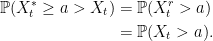The second equality here is using the reflection principle, so that X^r_t and X_t have the same distribution. On the other hand, on the event X_t ≥ a we necessarily have X^∗_t ≥ a,

Using addition of probabilities,

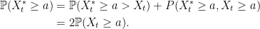This answers our original question of the distribution of X^∗_t. Its probability density will be twice that of X_t over x > 0 which, being normal with variance t, is

Conveniently, by symmetry of the normal distribution, the same holds for the absolute value |X_t| giving the simple result that it has the same distribution as X^∗_t.

Lemma 1 If X is standard Brownian motion, then X^∗_t has the same distribution as |X_t| for each time t ≥ 0.

In fact, we do not have to use the reflection principle in the form described above. While it is a powerful technique, it is useful to know of different (but very similar) approaches.

• Use the reflection principle, so that X^∗_t > a if either X_t > a or X^r_t > a.
• Condition on the first time τ at which X hits a. If this is before time t then, by symmetry of the normal distribution, there will be a 50% chance of ending up above a at time t. So, ℙ(X_t > a) = ℙ(X^∗_t > a)/2.
• Define a function f: ℝ → ℝ such that f(x) = 1 for x < a and which is antisymmetric about a. That is, f(x) = -1 for x > a. Conditioning on the first time τ at which X hits a,  this antisymmetry ensures that
  

  so,

  (2)

  As f(X_t) = 1 when X_t < a we obtain

  This is easily rearranged to obtain the same result as above for the distribution of X^∗_t.

While the third approach looks a little more involved at first glance, it can be very useful when we want to do something more complicated such as simultaneously consider the maximum and minimum of the process, where we would otherwise have to consider all the different ways in which the process can hit upper and lower barrier in different orders.

---

Joint distribution of the maximum and terminal value

The reflection principle can be taken further to compute the joint distribution of the maximum X^∗_t and terminal values X_t of a Brownian motion. Consider the possibility that X increases to level a before dropping back below level b < a at time t. Using the notation introduced above, this is exactly the same as the reflected process X^r being above 2a – b at time t,

Combined with the fact that X^∗_t ≥ X_t, this is sufficient to completely determine their joint distribution. However, let us generalize this a bit to look at the expectation of an arbitrary function of the terminal value of X.

If f: ℝ → ℝ is any measurable function such that f(X_t) has finite expectation, we can use the equivalence between X^∗_t > a and X_t > a or X^r_t > a to obtain,

Using the fact that X_t = 2a – X^r_t whenever X^r_t > a, and that X and X^r have the same distribution, we have proven the following result.

Theorem 2 If X is a standard Brownian motion and f: ℝ → ℝ is measurable such that f(X_t) has finite expectation, then

(3)

As explained above, there are alternative approaches which do not involve the reflected process X^r. Instead, we can reflect the function f to obtain a new function g: ℝ → ℝ which is antisymmetric about a.

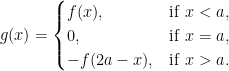Since g(X_t) = f(X_t) whenever X^∗_t < a, and antisymmetry about a ensures that identity (2) holds with g in place of f,

It is straightforward to rearrange this to obtain (3).

As X^∗ ≥ X, it is sufficient to apply (3) for the special case where f(x) = 0 on x > a, in which case it reduces to

The final equality here is just using symmetry of the normal distribution. So, restricting to the event X^∗_t > a has the same effect on the distribution of X_t as shifting it by 2a. At least, it does on the event {X_t ≤ a}. However, taking the expectation with respect to a shifted normal is the same as multiplying the integrand by an exponential term,

This can be determined by writing out the integrals with respect to the normal density and checking that they agree. Up to the constant normalizing factor, this is

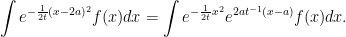Alternatively, a standard change of measure formula for the normal distribution can be used.

We have evaluated the probability that X^∗_t > a conditional on the value of X_t.

Theorem 3 Let X be a standard Brownian motion and t > 0 be a positive time. Then, for a > 0,

whenever X_t ≤ a.

As a special case, this directly gives the distribution of the maximum of a Brownian bridge simply by conditioning on X₁ = 0.

Corollary 4 If X_t is a Brownian bridge over 0 ≤ t ≤ 1 then,

over a ≥ 0.

The result stated for the Brownian bridge maximum is known as the Rayleigh distribution with scale parameter 1/2, and is the square root of an exponential distribution.

We can also ask about the maximum of a Brownian motion with drift μ, so that X_t = B_t + μt where B is standard Brownian motion. Interestingly, the drift has no effect whatsoever on the joint distribution of {X_s}_s ≤ t conditioned on X_t and, in particular, it has no effect on the distribution of X^∗_t conditioned on X_t. Hence, theorem 3 still holds. We saw in the post on Brownian bridges

where the second term on the right hand side is a Brownian bridge independently of the first term so that, conditioned on X_t, does not depend on the drift μ.

So, if X is a Brownian motion with drift μ, and f: ℝ → ℝ is a measurable function with f(x) = 0 over x > a, applying theorem 3 gives

The second equality here can be verified, as above, by integrating with respect to the normal density with mean μt for X_t, or by using standard change of measure formulas for the normal distribution. Adding on the nonzero values of f(X_t) over X_t > a, we obtain the generalization of theorem 2 to Brownian motion with drift.

Theorem 5 Let X be Brownian motion with drift μ and f: ℝ → ℝ be measurable such that f(X_t) is integrable. Then,

for all a > 0.

The final equality here is just using the fact that X_t has mean μt and, by symmetry, has the same distribution as 2μt – X_t.

---

Applications to non-Brownian motions

It is interesting to apply the ideas discussed above to processes which are not Brownian motion. While this does not exactly work, it does sometimes lead to inequalities which can be useful.

Consider a (cadlag) symmetric Lévy process X started from zero. For example, it could be a Cauchy process. This has independent and symmetric increments just as with Brownian motion, which is enough to conclude by the strong Markov property that the reflected process has the same distribution as X. However, it is not continuous. As a result, if τ is the first time at which it hits level a, we have X_τ ≥ a but equality need not hold. It is possible for the process to jump straight past the level, so that X_τ is strictly greater than a. So, it is possible for both X and the reflected process X^r to end up above a giving an inequality,

Applying the argument above results in

showing that, although X^∗_t need not have the same distribution as |X_t|, it is stochastically dominated by it.

For another example, suppose that X is an Ornstein-Uhlenbeck process, which is a solution to the stochastic differential equation (SDE)

for positive constants σ, λ and driving Brownian motion W. Such processes are strong Markov such that for times s < t then, conditioned on ℱ_s, X_t is normal with mean e^{–λ(t - s)}X_s and variance σ²(1 - e^{-2λ(t - s)})/(2λ). I will suppose that X starts from zero so that its distribution is a zero mean Gaussian at positive times.

If τ is the first time at which X reaches positive level a then, by continuity, we do have X_τ = a. However, its reflection at this time will not have the same distribution as X. For one thing, according to the SDE, X has negative drift –λa just after this time whereas X^r will have positive drift λa. So, the reflection principle does not work in the same way.

While it is possible to use a comparison between SDEs with different drifts to show that X^r stochastically dominates X, and continue in this way, a simpler argument can be used. As with the second bullet point further up in this post, we instead condition on ℱ_τ restricted to the event τ ≤ t. The strong Markov property says that X_t is normal with mean e^{–λ(t - τ)}a ≤ a, so we obtain

Multiplying through by twice the probability that τ ≤ t and, noting that this event is the same as X^∗_t ≥ a gives

So X^∗_t stochastically dominates |X_t|, in contrast to the Lévy process example above.

For a third example consider solutions to an SDE of the form

for driving Brownian motion W. Such processes are familiar in finance where X is the evolution of an asset price with local volatility surface σ(t, x). Now suppose that σ(t, x) is increasing in x at each time. It can be shown that this skews the distribution so that, for any starting value of X₀ we have

This can be explained intuitively. As the volatility is higher when X > X₀, this will make it more quickly move back below X₀ where the volatility is lower, so that it will stay below X₀ for longer. Hence, at a fixed positive time, it is more likely to be below X₀ than above it.

If we condition on the first time τ at which it reaches level a > X₀, then the forward starting process X_τ + s starts from level a and satisfies an SDE of the form above. So, conditioned on τ < t, this gives

Multiplying through by twice the probability that τ ≤ t we again obtain the inequality

As X does not have a symmetric distribution, this cannot be expressed in terms of X^∗_t stochastically dominating |X_t|, but the inequality is just as useful in this form. In the local volatility model used in finance, this is saying that with upwards sloping volatilities, the price of a one-touch option (paying 1 unit if X exceeds a at any time before expiry t) is more than twice as expensive as a digital call option (paying 1 unit if X exceeds a at time t). If the local volatility surface is decreasing in x instead, then the inequality goes the other way.