The Brownian Drawdown Process

The drawdown of a stochastic process is the amount that it has dropped since it last hit its maximum value so far. For process X with running maximum X^∗_t = sup_s ≤ tX_s, the drawdown is thus X^∗_t – X_t, which is a nonnegative process. This is as in figure 1 below.

The previous post used the reflection principle to show that the maximum of a Brownian motion has the same distribution as its terminal absolute value. That is, X^∗_t and |X_t| are identically distributed.

For a process X started from zero, its maximum and drawdown can be written as X^∗_t – X₀ and X^∗_t – X_t. Reversing the process in time across the interval [0, t] will exchange these values. So, reversing in time and translating so that it still starts from zero will exchange the maximum value and the drawdown. Specifically, write

for time index 0 ≤ s ≤ t. The maximum of Y is equal to the drawdown of X,

If X is standard Brownian motion then so is Y, since the independent normal increments property for Y follows from that of X. As already stated, the maximum Y^∗_t = X^∗_t – X_t has the same distribution as the absolute value |Y_t|= |X_t|. So, the drawdown has the same distribution as the absolute value at each time.

Lemma 1 If X is standard Brownian motion, then X^∗_t – X_t has the same distribution as |X_t| at each time t ≥ 0.

This equivalence of distributions can be taken much further. Whereas the post on the reflection principle only compared distributions at fixed times, it turns out that the joint distributions of the entire drawdown process are equivalent to those of the reflecting Brownian motion |X|. Certainly, this is far from true for the running maximum X^∗ which is increasing and never hits zero after time 0, in contrast to |X| which is never increasing over any nontrivial time intervals, and hits 0 every time that X changes sign. On the other hand, the drawdown X^∗ – X moves along with the Brownian motion –X except for the times at which X hits a maximum, in which case the drawdown hits 0. This is qualitatively similar to the paths of a reflecting Brownian motion, and we can show that they are identically distributed.

The idea is to show that both the absolute value and drawdown of a Brownian motion are Markov with the same transition probabilities, from which it follows that they have the same joint distribution. This requires looking at the distribution of the drawdown of X started at each positive time s > 0. However, the maximum value of the forward started paths Y_t = X_s + t are not the same as the forward started paths of X^∗, since the latter also maximizes over the values of X_u for u < s. Instead, we have X^∗_s + t = X^∗_s ∨ Y^∗_t. For this reason, we need a generalization of lemma 1 where the running maximum of the process is itself maxed with an independent value.

Consider fixing a value M ≥ 0, which could represent the maximum value of X at time zero (e.g., if there was some history of the process before time 0 with this value). So, the running maximum of X will be replaced by M ∨ X^∗ and the drawdown is replaced by M ∨ X^∗ – X. Lemma 1 continues across to this case.

Lemma 2 If X is standard Brownian motion and M ≥ 0 is a fixed value, then M ∨ X^∗_t – X_t has the same distribution as |M – X_t| at each time t ≥ 0.

This can be proved as an extension of lemma 1, noting first that processes Y_s = M ∨ X^∗_s – X_s and Z_s = |M – X_s| are equivalent up until the first time at which X hits level M. Denoting this time by τ = inf{s ≥ 0: X_s ≥ M}, then Y_t = Z_t on the event that τ ≥ t. On the other hand, conditioning on any value of τ < t, the strong Markov property says that X̃_s = X_τ + s – X_τ is a Brownian motion and, hence, lemma 1 says that Y_t = X̃^∗_t - τ – X̃_t - τ and Z_t = |X̃_t - τ| have the same distribution, proving lemma 2.

In the post on the reflection principle we spent some time constructing the joint distribution of X^∗_t and X_t. Now, when looking at the distributions of X^∗_t – X_t and M ∨ X^∗_t – X_t, we did not use that result and, instead, employed a time reversal trick. We could, of course, have used the joint distribution as expressed by theorems 2 or 3 of that post instead. It was just illuminating to see how a simple time reversal converts the maximum process X^∗ into the drawdown X^∗ – X, so that lemma 1 is clearly equivalent to the result that X^∗_t and |X_t| have the same distribution.

As it is good to have multiple methods of approaching a problem, let us also look at how the drawdown distribution also follows from the known joint distribution of X^∗_t and X_t. Setting Y_t = M ∨ X^∗_t – X_t, theorem 3 of the previous post gives

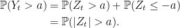
This holds on the event M – X_t ≤ a otherwise, when M – X_t > a, we automatically have Y_t > a. So, setting Z_t = M – X_t and taking expectations,

By either writing out the integral with respect the the normal density in the second term on the right hand side, or by applying a change of measure which shifts the mean of Z_t by 2a, this gives

Hence, Y_t and |Z_t| have the same distribution, giving a second proof of lemma 2.

Finally, we can make use of the drawdown distribution as expressed in lemma 2 to find its joint distribution.

Theorem 3 If X is standard Brownian motion, then X^∗_t – X_t and |X_t| have identical joint distributions over 0 ≤ t < ∞.

To prove this, it is sufficient to show that both processes are Markov with respect to the natural filtration ℱ_· of X, with the same transition probabilities and initial state. So, for times s < t, we need to show that the distribution of Y_t = X^∗_t – X_t conditioned on ℱ_s depends only on Y_s in the same way that the conditional distribution of Z_t = |X_t| depends on Z_s.

Considering the standard Brownian motion X̃_u = X_s + u – X_s, which is independent of ℱ_s, we have

so, by lemma 2 with X^∗_s – X_s in place of M, X̃ in place of X, and t – s in place of t, this has the same distribution as |(X^∗_s - X_s) – X̃_t - s|= |X^∗_s – X_t| when conditioned on ℱ_s. This is the absolute value of a normal with mean Y_s and variance t – s.

From the definition of Brownian motion, Z_t conditioned on ℱ_s is the absolute value of a normal with mean Z_s and variance t – s. This shows that Y and Z are both Markov with the same transition probabilities and with starting state Y₀ = Z₀ = 0, proving theorem 3. In fact, we did not make any use of the initial states of Y, Z other than that they are equal, so the exact same argument holds if we set Y_t = M ∨ X^∗_t – X_t and Z_t = |X_t – M| giving the following generalization.

Theorem 4 If X is standard Brownian motion and M ≥ 0 is a constant, then M ∨ X^∗_t – X_t and |M – X_t| have identical joint distributions over 0 ≤ t < ∞.