
If X is standard Brownian motion, what is the distribution of its absolute maximum |X|t∗ = sups ≤ t|Xs| over a time interval [0, t]? Previously, I looked at how the reflection principle can be used to determine that the maximum Xt∗ = sups ≤ tXs has the same distribution as |Xt|. This is not the same thing as the maximum of the absolute value though, which is a more difficult quantity to describe. As a first step, |X|t∗ is clearly at least as large as Xt∗ from which it follows that it stochastically dominates |Xt|.
I would like to go further and precisely describe the distribution of |X|t∗. What is the probability that it exceeds a fixed positive level a? For this to occur, the suprema of both X and –X must exceed a. Denoting the minimum and maximum by
 |
then |X|t∗ is the maximum of XtM and –Xtm. I have switched notation a little here, and am using XM to denote what was previously written as X∗. This is just to use similar notation for both the minimum and maximum. Using inclusion-exclusion, the probability that the absolute maximum is greater than a level a is,
 |
As XtM has the same distribution as |Xt| and, by symmetry, so does –Xm, we obtain
 |
This hasn’t really answered the question. All we have done is to re-express the probability in terms of both the minimum and maximum being beyond a level. For large values of a it does, however, give a good approximation. The probability of the Brownian motion reaching a large positive value a and then dropping to the large negative value –a will be vanishingly small, so the final term in the identity above can be neglected. This gives an asymptotic approximation as a tends to infinity,
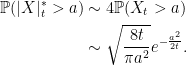 |
(1) |
The last expression here is just using the fact that Xt is centered Gaussian with variance t and applying a standard approximation for the cumulative normal distribution function.
For small values of a, approximation (1) does not work well at all. We know that the left-hand-side should tend to 1, whereas 4ℙ(Xt > a) will tend to 2, and the final expression diverges. In fact, it can be shown that
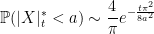 |
(2) |
as a → 0. I gave a direct proof in this math.stackexchange answer. In this post, I will look at how we can compute joint distributions of the minimum, maximum and terminal value of Brownian motion, from which limits such as (2) will follow.
Distribution of the Minimum and Maximum
For a < 0 < b, we look at the event that standard Brownian motion X does not reach either of these levels before a fixed positive time t, and compute its probability. As explained in the post on the reflection principle, there are different ways of approaching such problems. While it is possible to apply the reflection principle here, giving an intuitive ‘pathwise’ approach to the solution, it can get a bit messy to go through the details. It is necessary to reflect through both levels, which can occur arbitrarily many times, and use an infinite inclusion-exclusion sequence to avoid over-counting any possibilities. Instead, I will take a more mathematically straightforward approach using the ‘square wave’ function g: ℝ → ℝ,
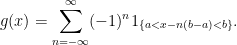 |
This is equal to 1 on the interval (a, b), and is antisymmetric about both a and b,
 |
If τ is the first time at which X hits a or b then, by the strong Markov property Xτ + s – Xτ is standard Brownian motion independently of ℱτ. Consequently,conditioned on τ ≤ t, Xt – Xτ has a symmetric distribution and, by antisymmetry of g about the level Xτ, g(Xt) has zero expectation. On the other hand, if τ > t then Xt is in the interval (a, b), so g(Xt) = 1 giving,
![\displaystyle \begin{aligned} {\mathbb E}[g(X_t)]&={\mathbb E}[1_{\{\tau > t\}}g(X_t)]+{\mathbb E}[1_{\{\tau\le t\}}g(X_t)]\\ &={\mathbb P}(\tau > t)+0. \end{aligned}](https://s0.wp.com/latex.php?latex=%5Cdisplaystyle++%5Cbegin%7Baligned%7D+%7B%5Cmathbb+E%7D%5Bg%28X_t%29%5D%26%3D%7B%5Cmathbb+E%7D%5B1_%7B%5C%7B%5Ctau+%3E+t%5C%7D%7Dg%28X_t%29%5D%2B%7B%5Cmathbb+E%7D%5B1_%7B%5C%7B%5Ctau%5Cle+t%5C%7D%7Dg%28X_t%29%5D%5C%5C+%26%3D%7B%5Cmathbb+P%7D%28%5Ctau+%3E+t%29%2B0.+%5Cend%7Baligned%7D+&bg=ffffff&fg=000000&s=0&c=20201002) |
As τ > t is equivalent to a < Xtm and XtM < b, plugging in the definition of g above in the expectation on the left hand side expresses the joint distribution of Xtm, XtM in terms of the normally distributed Xt.
Theorem 1 If X is standard Brownian motion, t is a fixed positive time and a < 0 < b are fixed levels then,

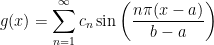
This idea can be taken further to compute the joint distribution of Xtm, XtM, Xt. For any integrable function f: (a, b) → ℝ, there is a unique g: ℝ → ℝ equal to f on the interval (a, b) and antisymmetric about both a and b. Note that reflecting about both these levels in turn is the same as translating by 2(b - a), so g must be periodic with period 2(b - a). It can be explicitly constructed as
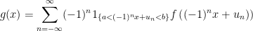 |
(3) |
where I am setting un = n(b - a) for n even and un = n(b - a) + a + b for n odd. Writing it in this way will be useful for our application, although it may not be immediately obvious that it satisfies the required conditions. To see that it is antisymmetric about a, it can be checked that reflecting x through this level exchanges terms n = 2m and n = 2m – 1 in the sum whilst flipping their sign, and reflecting through b exchanges n = 2m and n = 2m + 1 with opposite signs.
If τ is the first time when X hits either a or b then, using exactly the same argument as above, antisymmetry about both a and b implies that the expectation of g(Xt) conditioned on τ ≤ t is zero, and g(Xt) = f(Xt) on τ > t,
![\displaystyle {\mathbb E}[g(X_t)]={\mathbb E}[1_{\{\tau > t\}}f(X_t)]](https://s0.wp.com/latex.php?latex=%5Cdisplaystyle++%7B%5Cmathbb+E%7D%5Bg%28X_t%29%5D%3D%7B%5Cmathbb+E%7D%5B1_%7B%5C%7B%5Ctau+%3E+t%5C%7D%7Df%28X_t%29%5D+&bg=ffffff&fg=000000&s=0&c=20201002) |
Plugging in the expression above for g gives us the joint distribution of Xtm, XtM, Xt.
Theorem 2 If X is standard Brownian motion, t is a fixed positive time, a < 0 < b are fixed levels and f: (a, b) → ℝ is integrable then,
(4) where un = n(b - a) for n even and un = n(b - a) + a + b for n odd.
![\displaystyle \begin{aligned} &{\mathbb E}\left[1_{\{a < X_t^m,X_t^M < b\}}f(X_t)\right]\\ &=\sum_{n=-\infty}^\infty(-1)^n{\mathbb E}\left[1_{\{a < X_t+u_n < b\}}f\left(X_t+u_n\right)\right] \end{aligned}](https://s0.wp.com/latex.php?latex=%5Cdisplaystyle++%5Cbegin%7Baligned%7D+%26%7B%5Cmathbb+E%7D%5Cleft%5B1_%7B%5C%7Ba+%3C+X_t%5Em%2CX_t%5EM+%3C+b%5C%7D%7Df%28X_t%29%5Cright%5D%5C%5C+%26%3D%5Csum_%7Bn%3D-%5Cinfty%7D%5E%5Cinfty%28-1%29%5En%7B%5Cmathbb+E%7D%5Cleft%5B1_%7B%5C%7Ba+%3C+X_t%2Bu_n+%3C+b%5C%7D%7Df%5Cleft%28X_t%2Bu_n%5Cright%29%5Cright%5D+%5Cend%7Baligned%7D+&bg=ffffff&fg=000000&s=0&c=20201002)
Here, the expectations on the right hand side are just the summand in (3) with Xt replacing x. By symmetry of the normal distribution, I also replaced (-1)nXt by Xt to simplify the expression.
The expectations on the right hand side of (4) can be rearranged. For any integrable function h, using the fact that Xt is normal with zero mean and variance t,
![\displaystyle {\mathbb E}[h(X_t+u)] ={\mathbb E}\left[e^{\frac{u}{t}X_t-\frac{u^2}{2t}}h(X_t)\right].](https://s0.wp.com/latex.php?latex=%5Cdisplaystyle++%7B%5Cmathbb+E%7D%5Bh%28X_t%2Bu%29%5D+%3D%7B%5Cmathbb+E%7D%5Cleft%5Be%5E%7B%5Cfrac%7Bu%7D%7Bt%7DX_t-%5Cfrac%7Bu%5E2%7D%7B2t%7D%7Dh%28X_t%29%5Cright%5D.+&bg=ffffff&fg=000000&s=0&c=20201002) |
This is just the standard measure change for translating a normal density. Applying this to the expectations in the summation on the right hand side of (4) gives,
![\displaystyle \begin{aligned} &{\mathbb E}\left[1_{\{a < X_t^m,X_t^M < b\}}f(X_t)\right]\\ &=\sum_{n=-\infty}^\infty(-1)^n{\mathbb E}\left[e^{\frac{u_n}{t}X_t-\frac{u_n^2}{2t}}1_{\{a < X_t < b\}}f\left(X_t)\right)\right]. \end{aligned}](https://s0.wp.com/latex.php?latex=%5Cdisplaystyle++%5Cbegin%7Baligned%7D+%26%7B%5Cmathbb+E%7D%5Cleft%5B1_%7B%5C%7Ba+%3C+X_t%5Em%2CX_t%5EM+%3C+b%5C%7D%7Df%28X_t%29%5Cright%5D%5C%5C+%26%3D%5Csum_%7Bn%3D-%5Cinfty%7D%5E%5Cinfty%28-1%29%5En%7B%5Cmathbb+E%7D%5Cleft%5Be%5E%7B%5Cfrac%7Bu_n%7D%7Bt%7DX_t-%5Cfrac%7Bu_n%5E2%7D%7B2t%7D%7D1_%7B%5C%7Ba+%3C+X_t+%3C+b%5C%7D%7Df%5Cleft%28X_t%29%5Cright%29%5Cright%5D.+%5Cend%7Baligned%7D+&bg=ffffff&fg=000000&s=0&c=20201002) |
This gives the joint distribution of Xtm, XtM conditioned on Xt.
Theorem 3 If X is standard Brownian motion, t is a fixed positive time, a < 0 < b are fixed levels then,
for a < Xt < b, where un = n(b - a) for n even and un = n(b - a) + a + b for n odd.
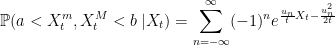
In particular, taking b = –a gives the distribution of the absolute maximum conditioned on the terminal value.
Corollary 4 If X is standard Brownian motion, t is a fixed positive time and a > 0 is a fixed level then,
for |Xt|< a, where un = 2na.

Conditioning on Xt = 0 also gives the distribution of the absolute maximum of a Brownian bridge.
Corollary 5 If X is a standard Brownian bridge and a > 0 is a fixed level then,

Transformed Sums
The sums given in theorems 1,2,3 and corollaries 4,5 all converge quickly in n. This is especially true for large absolute values of a and b where very few terms are needed to get an accurate approximation. On the other hand, for small values of a and b, a lot of terms may be needed before the convergence kicks in, so is not so useful in this case. I now look at how these can be transformed to give a sum where only a small number of terms will be needed for small absolute values of a and b. This is essentially a Jacobi identity, proved using Fourier series.
As the function g defined by (3) is periodic, it can be written as a Fourier series which consists of terms of the form exp(iπnx/(b - a)). Since expectations of exp(iπnXt/(b - a)) have a simple closed form expression, this removes the summation from (4) replacing it, instead, with the Fourier expansion. Actually, antisymmetry says that g can be written as a sine series,
 |
with coefficients,
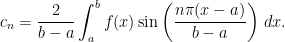 |
(5) |
The expectation of the sine of a normal variable of mean μ and variance ν is
![\displaystyle {\mathbb E}[\sin(U)]=e^{-\frac\nu2}\sin(\mu),](https://s0.wp.com/latex.php?latex=%5Cdisplaystyle++%7B%5Cmathbb+E%7D%5B%5Csin%28U%29%5D%3De%5E%7B-%5Cfrac%5Cnu2%7D%5Csin%28%5Cmu%29%2C+&bg=ffffff&fg=000000&s=0&c=20201002) |
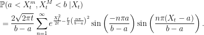
So, we can take expectations of the sine expansion of g(Xt) to obtain a description of the joint distribution of the maximum, minimum and terminal value of a Brownian motion in the same way as for theorem 2 above.
Theorem 6 If X is standard Brownian motion, t is a fixed positive time, a < 0 < b are fixed levels and f: (a, b) → ℝ is integrable then,
(6) where cn are given by (5).
![\displaystyle {\mathbb E}\left[1_{\{a < X_t^m,X_t^M < b\}}f(X_t)\right]=\sum_{n=1}^\infty c_n e^{-\frac t2\left(\frac{n\pi}{b-a}\right)^2}\sin\left(\frac{-n\pi a}{b-a}\right)](https://s0.wp.com/latex.php?latex=%5Cdisplaystyle++%7B%5Cmathbb+E%7D%5Cleft%5B1_%7B%5C%7Ba+%3C+X_t%5Em%2CX_t%5EM+%3C+b%5C%7D%7Df%28X_t%29%5Cright%5D%3D%5Csum_%7Bn%3D1%7D%5E%5Cinfty+c_n+e%5E%7B-%5Cfrac+t2%5Cleft%28%5Cfrac%7Bn%5Cpi%7D%7Bb-a%7D%5Cright%29%5E2%7D%5Csin%5Cleft%28%5Cfrac%7B-n%5Cpi+a%7D%7Bb-a%7D%5Cright%29+&bg=ffffff&fg=000000&s=0&c=20201002)
This is a fast converging sequence and, when b – a is small very few terms will be required for an accurate approximation.
Computing the coefficients for f = 1,
 |
gives an alternative expression for the distribution of the minimum and maximum from that in theorem 1.
Theorem 7 If X is standard Brownian motion, t is a fixed positive time and a < 0 < b are fixed levels then,

Applying this with a = –b gives an expression for the distribution of the absolute maximum.
Corollary 8 If X is standard Brownian motion, t is a fixed positive time and a > 0 is a fixed level then,
Looking again at expression (6), substituting in the integral (5) for the sine components and commuting summation with the integration,
![\displaystyle {\mathbb E}\left[1_{\{a < X_t^m,X_t^M < b\}}f(X_t)\right]=\int_a^b p(x)f(x)\,dx](https://s0.wp.com/latex.php?latex=%5Cdisplaystyle++%7B%5Cmathbb+E%7D%5Cleft%5B1_%7B%5C%7Ba+%3C+X_t%5Em%2CX_t%5EM+%3C+b%5C%7D%7Df%28X_t%29%5Cright%5D%3D%5Cint_a%5Eb+p%28x%29f%28x%29%5C%2Cdx+&bg=ffffff&fg=000000&s=0&c=20201002) |
where
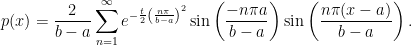 |
To compute the probability conditioned on Xt, we just divide by its probability density, giving a transformed version of theorem 3.
Theorem 9 If X is standard Brownian motion, t is a fixed positive time, a < 0 < b are fixed levels then,
(7) for a < Xt < b.
Taking b = –a gives the distribution of the absolute maximum conditioned on the terminal value. Doing this, the product of sines on the right hand side of (7) is
 |
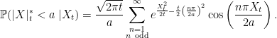
We obtain the transformed version of corollary 4 for the distribution of the absolute maximum of X conditioned on its terminal value.
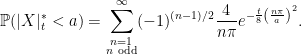
Corollary 10 If X is standard Brownian motion, t is a fixed positive time and a > 0 is a fixed level then,
for |Xt|< a.
Finally, conditioning on Xt = 0 gives the transformed version of corollary 5 for the absolute maximum of a Brownian bridge.
Corollary 11 If X is a standard Brownian bridge and a > 0 is a fixed level then,


Thank you very much for the very clear explanations (better than other materials I have consulted). I am heavily using these developments for academic purposes. May I ask which reference you recommend for citing these? In particular the equation in Corollary 10 which I cannot find in any text book.
Hi Mohsen. I simply worked out formulas in this page myself, although they are well-known. I expect that the 2001 paper “Probability laws related to the Jacobi theta and Riemann zeta functions, and Brownian excursions” by Biane, Pitman, and Yor will either contain what you need, or have the relevant references, as it relies on this stuff.
https://doi.org/10.1090/S0273-0979-01-00912-0
Good luck!
Hi,
Great post! Thank you very much.
The Theorem 7 looks to me like Theorem 3 viewed through the lens of the Poisson summation formula.
AR
It is! I mentioned that this is essentially a Jacobi identity (by which, I mean the Poisson summation formula, since it is an identity of Jacobi theta functions). Might edit in the words Poisson summation formula when I have time
Happy new year!
I think there is catch in your formula for $u_n$ for odd values of $n$. It should either be $u_n = n (b-a) + 2a$ or $u_n = n(b-a) + 2b$ but not $u_n = n(b-a) + b+a$.
It is not a proof but your formula for the trivariate distribution of the max, min is for instance not in line with that of the paper:
https://www.sciencedirect.com/science/article/abs/pii/S0167715212004749
But there are other evidences such as broken symmetries against your $b+a$ formula.
Cheers
AR
Hi, Happy new year!
I just compared my formula from theorem 3 above with the one in the introduction of the paper you linked, and they agree. This is using the substitution n=2k for n even and n=2k+1 for n odd.
u_n = 2k(b-a)+2b = (2k+1)(b-a)+a+b=n(b-a)+a+b
You are right. Sorry. There is still something I do not quite get in both your version and that of the paper then. 🙂
Consider a function f from [0, 1]. You want to make it odd, you create O(f) on [-1, 1] such that O(f)(u) = f(u) on [0, 1] and O(f)(u) = -f(-u) on [-1, 0].
You can now periodize it OP(f)(u) = sum(O(f)(u-2n); n in Z) to make it antisymmetric about any integer.
If you work on [a,b] with F, you can just use u = (x-a)/(b-a) and x = a +(b-a)u giving you:
f(u) = F(a + (b-a)u)
and lift F into the f world to use the OP operator:
OP(F)(x) =OP(f)((x-a)/(b-a)) = sum(O(f)((x-a)/(b-a)-2n); n in Z)
I would have expected that taking the expectation as you did and Girsanoving the results should have boiled down to applying the following changes of variables:
(y-a)/(b-a) = (x-a)/(b-a)-2n i.e. y = x – 2n (b-a) for the unreflected class
(y-a)/(b-a) = -((x-a)/(b-a)-2n) i.e. y = -(x – 2a – 2n(b-a)) for the reflected one
The goal would indeed be to recast everything in terms of the original function F in the two subcases:
O(f)((x-a)/(b-a)-2n) = f((y-a)/(b-a)) = F(y)
O(f)((x-a)/(b-a)-2n) = -f(-(y-a)/(b-a)) = -F(y)
And therefore it would rather have led to u_n = 2n(b-a) for even indices and u_n = 2n(b-a) + 2a
What did I miss?
Arnaud Rivoira
Sorry again. Yes, now I realize that your answer solved indeed the puzzle. I was wrong thinking that for even indices and
  for odd ones. It was indeed
  and
and 