
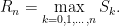
Spitzer’s formula is a remarkable result giving the precise joint distribution of the maximum and terminal value of a random walk in terms of the marginal distributions of the process. I have already covered the use of the reflection principle to describe the maximum of Brownian motion, and the same technique can be used for simple symmetric random walks which have a step size of ±1. What is remarkable about Spitzer’s formula is that it applies to random walks with any step distribution.
We consider partial sums
 |
for an independent identically distributed (IID) sequence of real-valued random variables X1, X2, …. This ranges over index n = 0, 1, … starting at S0 = 0 and has running maximum
 |
Spitzer’s theorem is typically stated in terms of characteristic functions, giving the distributions of (Rn, Sn) in terms of the distributions of the positive and negative parts, Sn+ and Sn–, of the random walk.
Theorem 1 (Spitzer) For α, β ∈ ℝ,
(1) where ϕn, wn are the characteristic functions
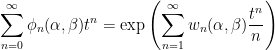
![\displaystyle \begin{aligned} \phi_n(\alpha,\beta)&={\mathbb E}\left[e^{i\alpha R_n+i\beta(R_n-S_n)}\right],\\ w_n(\alpha,\beta)&={\mathbb E}\left[e^{i\alpha S_n^++i\beta S_n^-}\right]\\ &={\mathbb E}\left[e^{i\alpha S_n^+}\right]+{\mathbb E}\left[e^{i\beta S_n^-}\right]-1. \end{aligned}](https://s0.wp.com/latex.php?latex=%5Cdisplaystyle+%5Cbegin%7Baligned%7D+%5Cphi_n%28%5Calpha%2C%5Cbeta%29%26%3D%7B%5Cmathbb+E%7D%5Cleft%5Be%5E%7Bi%5Calpha+R_n%2Bi%5Cbeta%28R_n-S_n%29%7D%5Cright%5D%2C%5C%5C+w_n%28%5Calpha%2C%5Cbeta%29%26%3D%7B%5Cmathbb+E%7D%5Cleft%5Be%5E%7Bi%5Calpha+S_n%5E%2B%2Bi%5Cbeta+S_n%5E-%7D%5Cright%5D%5C%5C+%26%3D%7B%5Cmathbb+E%7D%5Cleft%5Be%5E%7Bi%5Calpha+S_n%5E%2B%7D%5Cright%5D%2B%7B%5Cmathbb+E%7D%5Cleft%5Be%5E%7Bi%5Cbeta+S_n%5E-%7D%5Cright%5D-1.+%5Cend%7Baligned%7D+&bg=ffffff&fg=000000&s=0&c=20201002)
As characteristic functions are bounded by 1, the infinite sums in (1) converge for |t|< 1. However, convergence is not really necessary to interpret this formula, since both sides can be considered as formal power series in indeterminate t, with equality meaning that coefficients of powers of t are equated. Comparing powers of t gives
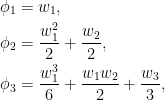 |
(2) |
and so on.
Spitzer’s theorem in the form above describes the joint distribution of the nonnegative random variables (Rn, Rn - Sn) in terms of the nonnegative variables (Sn+, Sn–). While this does have a nice symmetry, it is often more convenient to look at the distribution of (Rn, Sn) in terms of (Sn+, Sn), which is achieved by replacing α with α + β and β with –β in (1). This gives a slightly different, but equivalent, version of the theorem.
Theorem 2 (Spitzer) For α, β ∈ ℝ,
(3) where ϕ̃n, w̃n are the characteristic functions

![\displaystyle \begin{aligned} \tilde\phi_n(\alpha,\beta)&={\mathbb E}\left[e^{i\alpha R_n+i\beta S_n}\right],\\ \tilde w_n(\alpha,\beta)&={\mathbb E}\left[e^{i\alpha S_n^++i\beta S_n}\right]. \end{aligned}](https://s0.wp.com/latex.php?latex=%5Cdisplaystyle+%5Cbegin%7Baligned%7D+%5Ctilde%5Cphi_n%28%5Calpha%2C%5Cbeta%29%26%3D%7B%5Cmathbb+E%7D%5Cleft%5Be%5E%7Bi%5Calpha+R_n%2Bi%5Cbeta+S_n%7D%5Cright%5D%2C%5C%5C+%5Ctilde+w_n%28%5Calpha%2C%5Cbeta%29%26%3D%7B%5Cmathbb+E%7D%5Cleft%5Be%5E%7Bi%5Calpha+S_n%5E%2B%2Bi%5Cbeta+S_n%7D%5Cright%5D.+%5Cend%7Baligned%7D+&bg=ffffff&fg=000000&s=0&c=20201002)
Taking β = 0 in either (1) or (3) gives the distribution of Rn in terms of Sn+,
![\displaystyle \sum_{n=0}^\infty {\mathbb E}\left[e^{i\alpha R_n}\right]t^n=\exp\left(\sum_{n=1}^\infty {\mathbb E}\left[e^{i\alpha S_n^+}\right]\frac{t^n}n\right)](https://s0.wp.com/latex.php?latex=%5Cdisplaystyle+%5Csum_%7Bn%3D0%7D%5E%5Cinfty+%7B%5Cmathbb+E%7D%5Cleft%5Be%5E%7Bi%5Calpha+R_n%7D%5Cright%5Dt%5En%3D%5Cexp%5Cleft%28%5Csum_%7Bn%3D1%7D%5E%5Cinfty+%7B%5Cmathbb+E%7D%5Cleft%5Be%5E%7Bi%5Calpha+S_n%5E%2B%7D%5Cright%5D%5Cfrac%7Bt%5En%7Dn%5Cright%29+&bg=ffffff&fg=000000&s=0&c=20201002) |
(4) |
I will give a proof of Spitzer’s theorem below. First, though, let’s look at some consequences, starting with the following strikingly simple result for the expected maximum of a random walk.
Corollary 3 For each n ≥ 0,
(5)
![\displaystyle {\mathbb E}[R_n]=\sum_{k=1}^n\frac1k{\mathbb E}[S_k^+].](https://s0.wp.com/latex.php?latex=%5Cdisplaystyle+%7B%5Cmathbb+E%7D%5BR_n%5D%3D%5Csum_%7Bk%3D1%7D%5En%5Cfrac1k%7B%5Cmathbb+E%7D%5BS_k%5E%2B%5D.+&bg=ffffff&fg=000000&s=0&c=20201002)
Proof: As Rn ≥ S1+ = X1+, if Xk+ have infinite mean then both sides of (5) are infinite. On the other hand, if Xk+ have finite mean then so do Sn+ and Rn. Using the fact that the derivative of the characteristic function of an integrable random variable at 0 is just i times its expected value, compute the derivative of (4) at α = 0,
![\displaystyle \begin{aligned} \sum_{n=0}^\infty i{\mathbb E}[R_n]t^n &=\exp\left(\sum_{n=1}^\infty \frac{t^n}n\right)\sum_{n=1}^\infty i{\mathbb E}[S_n^+]\frac{t^n}n\\ &=\exp\left(-\log(1-t)\right)\sum_{n=1}^\infty i{\mathbb E}[S_n^+]\frac{t^n}n\\ &=(1-t)^{-1}\sum_{n=1}^\infty i{\mathbb E}[S_n^+]\frac{t^n}n\\ &=(1+t+t^2+\cdots)\sum_{n=1}^\infty i{\mathbb E}[S_n^+]\frac{t^n}n. \end{aligned}](https://s0.wp.com/latex.php?latex=%5Cdisplaystyle+%5Cbegin%7Baligned%7D+%5Csum_%7Bn%3D0%7D%5E%5Cinfty+i%7B%5Cmathbb+E%7D%5BR_n%5Dt%5En+%26%3D%5Cexp%5Cleft%28%5Csum_%7Bn%3D1%7D%5E%5Cinfty+%5Cfrac%7Bt%5En%7Dn%5Cright%29%5Csum_%7Bn%3D1%7D%5E%5Cinfty+i%7B%5Cmathbb+E%7D%5BS_n%5E%2B%5D%5Cfrac%7Bt%5En%7Dn%5C%5C+%26%3D%5Cexp%5Cleft%28-%5Clog%281-t%29%5Cright%29%5Csum_%7Bn%3D1%7D%5E%5Cinfty+i%7B%5Cmathbb+E%7D%5BS_n%5E%2B%5D%5Cfrac%7Bt%5En%7Dn%5C%5C+%26%3D%281-t%29%5E%7B-1%7D%5Csum_%7Bn%3D1%7D%5E%5Cinfty+i%7B%5Cmathbb+E%7D%5BS_n%5E%2B%5D%5Cfrac%7Bt%5En%7Dn%5C%5C+%26%3D%281%2Bt%2Bt%5E2%2B%5Ccdots%29%5Csum_%7Bn%3D1%7D%5E%5Cinfty+i%7B%5Cmathbb+E%7D%5BS_n%5E%2B%5D%5Cfrac%7Bt%5En%7Dn.+%5Cend%7Baligned%7D+&bg=ffffff&fg=000000&s=0&c=20201002) |
Equating powers of t gives the result. ⬜
The expression for the distribution of Rn in terms of Sn+ might not be entirely intuitive at first glance. Sure, it describes the characteristic functions and, hence, determines the distribution. However, we can describe it more explicitly. As suggested by the evaluation of the first few terms in (2), each ϕn is a convex combination of products of the wn. As is well known, the characteristic function of the sum of random variables is equal to the product of their characteristic functions. Also, if we select a random variable at random from a finite set, then its characteristic function is a convex combination of those of the individual variables with coefficients corresponding to the probabilities in the random choice. So, (3) expresses the distribution of (Rn, Sn) as a random choice of sums of independent copies of (Sk+, Sk).
In fact, expressions such as (1,3) are common in many branches of maths, such as zeta functions associated with curves over finite fields. We have a power series which can be expressed in two different ways,
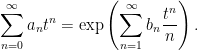 |
The left hand side is the generating function of the sequence an. The right hand side is a kind of zeta function associated with the sequence bn, and is sometimes referred to as the combinatorial zeta function. The logarithmic derivative gives Σnbntn-1, which is the generating function of bn+1.
The exponential formula explicitly describes coefficients an in terms of the bn,
 |
(6) |
Here, σ is a permutation of n elements and σk denotes the number of cycles of length k. Applying to Spitzer’s formula (1), this gives
 |
(7) |
As the characteristic function of a sum of independent random variables is the product of their characteristic functions, (7) gives the following construction for the distribution of (Rn, Sn). Let random permutation σ be uniform on Sym(σ). If its cycle lengths are l1, l2, …, lr then the term on the right of (7) corresponding to the permutation is wl1wl2⋯wlr. Hence, choosing an independent sequence of random variables Z1, …, Zr having the same distributions as Sl1, …, Slr then, (Rn, Rn - Sn) has the same distribution as
 |
or, equivalently, (Rn, Sn) has the same distribution as
 |
(8) |
This formulation makes it clear that 𝔼[Rn] is the sum of 𝔼[Sk+] weighted by the expected number of cycles of length k. Corollary 3 follows from the fact that the expected number of length k cycles of a random permutation in Sym(n) equals 1/k.
As an example application, consider the probability that the random walk is never positive for the first n steps or, equivalently, Rn = 0.
Lemma 4
Proof: Using the notation above,
![\displaystyle \begin{aligned} {\mathbb P}(R_n=0) &={\mathbb P}(Z_1^++\cdots+Z_r^+=0)\\ &={\mathbb E}[{\mathbb P}(Z_1\le0\vert\;\sigma)\cdots{\mathbb P}(Z_r\le0\vert\;\sigma)]. \end{aligned}](https://s0.wp.com/latex.php?latex=%5Cdisplaystyle+%5Cbegin%7Baligned%7D+%7B%5Cmathbb+P%7D%28R_n%3D0%29+%26%3D%7B%5Cmathbb+P%7D%28Z_1%5E%2B%2B%5Ccdots%2BZ_r%5E%2B%3D0%29%5C%5C+%26%3D%7B%5Cmathbb+E%7D%5B%7B%5Cmathbb+P%7D%28Z_1%5Cle0%5Cvert%5C%3B%5Csigma%29%5Ccdots%7B%5Cmathbb+P%7D%28Z_r%5Cle0%5Cvert%5C%3B%5Csigma%29%5D.+%5Cend%7Baligned%7D+&bg=ffffff&fg=000000&s=0&c=20201002) |
This is using the fact that, conditioned on the random permutation σ, Zk are independent. As Zk is distributed as Slk where lk is the length of the k‘th cycle and recalling that σk denotes the number of cycles of length k,
![\displaystyle {\mathbb P}(R_n=0)={\mathbb E}\left[{\mathbb P}(S_1\le0)^{\sigma_1}{\mathbb P}(S_2\le0)^{\sigma_2}\cdots{\mathbb P}(S_n\le0)^{\sigma_n}\right].](https://s0.wp.com/latex.php?latex=%5Cdisplaystyle+%7B%5Cmathbb+P%7D%28R_n%3D0%29%3D%7B%5Cmathbb+E%7D%5Cleft%5B%7B%5Cmathbb+P%7D%28S_1%5Cle0%29%5E%7B%5Csigma_1%7D%7B%5Cmathbb+P%7D%28S_2%5Cle0%29%5E%7B%5Csigma_2%7D%5Ccdots%7B%5Cmathbb+P%7D%28S_n%5Cle0%29%5E%7B%5Csigma_n%7D%5Cright%5D.+&bg=ffffff&fg=000000&s=0&c=20201002) |
Comparing with the exponential formula (6) gives the result. ⬜
For symmetric distributions, we obtain a simple and surprising result which does not depend on the specific random walk distribution.
Corollary 5 Suppose that the steps Xk of the random walk have a continuous symmetric distribution. Then,
for each n ≥ 0.

Proof: As Sk has a symmetric distribution and, by continuity, ℙ(Sk = 0) = 0, we obtain ℙ(Sk ≤ 0) = 1/2. Lemma 4 gives
 |
The final equality is just plugging in an explicit expression for the binomial coefficients and, equating powers of t, gives the result. ⬜
This result is sometimes known as the Sparre Anderson theorem, and there is a more direct proof which does not go via Spitzer’s formula. See section 2 of the 2012 paper Persistence of iterated partial sums by Dembo, Ding and Gao. The approach given there, though, does not provide a proof of the more general statement of lemma 4. Yet another method of proof is given in a 2010 paper by Satya Majumdar.
Returning to the discussion for the joint distribution, recall that the steps Xk of the random walk are IID. So, the sum of any number m of these has the same distribution as Sm, and sums over disjoint sets of indices are independent. This means that the terms Zj in (8) can be expressed as a sum of Xk as k ranges over lj values. It is convenient to allow it to range over the elements of the corresponding length-lj cycle, which partition {1, …, n} and, hence, the resulting terms Zj have the required distribution and sum to Sn.
Lemma 6 Using cyc(σ) to denote the set of cycles and writing
(9) then (R̃n, Sn) has the same distribution as (Rn, Sn).
In Spitzer’s original proof, lemma 6 was proved directly. This implies theorem 1 by applying the logic above in reverse. The proof is combinatorial and a bit tricky though. See the 1959 paper A combinatorial lemma and its application to probability theory by Spitzer. By contrast, the proof I will give below is of a very different nature and drops out from some straightforward algebra.
Instead of using (9) directly, it can be convenient to reorder the random walk increments Xk to be contiguous for each cycle.
Theorem 7 For fixed positive integer n, let
be a finite (random) length sequence of integer random variables such that τ0 – τ1, …, τm-1 – τm has the same distribution (up to order) as the cycle lengths of a uniformly random permutation of size n. If these are independent of the random walk Sk, set
Then (R̃n, Sn) has the same distribution as (Rn, Sn).

Proof: The set of differences lk = τk-1 – τk are distributed as the set of cycle lengths of a random permutation from Sym(n). By independence, conditioned on these, the increments Sτk-1 – Sτk are independent with the same distribution as Slk. So, the result follows from (8). ⬜
Constructing random times τk with the required property is not difficult. Starting with τ0 = n, for each k ≥ 0 in order:
- if τk > 0 then choose τk+1 uniformly over 0, 1, …, τk – 1.
- if τk = 0 then set m = k and terminate.
It can be seen that these have the required distribution using the following simple fact: for a random permutation σ ∈ Sym(n), the length of the cycle containing element 1 is uniform from 1 to n. We can choose n – τ1 to be the length of this cycle. Then, deleting the elements of this cycle, we have a random permutation of length τ1 and the remaining cycle lengths are chosen in the same way for this shorter permutation.
 |
|
Lévy Processes
The continuous-time counterpart of a random walks is a Lévy process. These are stochastic processes satisfying an IID increments property. Specifically, {St}t≥0 is a Lévy process if it has right-continuous sample paths and, for times s, t > 0, the increment St+s – St is independent of {Su: u ≤ t} and has distribution not depending on t. Choosing a time step h > 0, the discrete-time process S̃n = Snh is a random walk with IID increments Xn = Snh – S(n-1)h and the original Lévy process is recovered by taking h arbitrarily small. Examples include Poisson processes, Cauchy processes and, of course, Brownian motion.
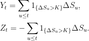
Spitzer’s formula and its consequences follow across to the continuous-time situation, as I will explain now. Throughout this section, St will be a real-valued Lévy process starting from S0 = 0 and its running maximum is denoted
 |
This section will be a straightforward run through of the results already stated above, and converting them to the continuous-time setting. I start with the continuous-time version of corollary 3, giving the expected value of the maximum of a Lévy process.
Lemma 8 For all t ≥ 0,
![\displaystyle {\mathbb E}[R_t]=\int_0^t{\mathbb E}[S_u^+]\frac{du}{u}.](https://s0.wp.com/latex.php?latex=%5Cdisplaystyle+%7B%5Cmathbb+E%7D%5BR_t%5D%3D%5Cint_0%5Et%7B%5Cmathbb+E%7D%5BS_u%5E%2B%5D%5Cfrac%7Bdu%7D%7Bu%7D.+&bg=ffffff&fg=000000&s=0&c=20201002)
Proof: By scaling time if necessary, without loss of generality we can take t = 1. Fixing integer n > 0, consider the random walk S̃k = Sk/n. Corollary 3 gives,
![\displaystyle {\mathbb E}\left[\sup_{k\le n}S_{k/n}\right]=\sum_{k=1}^n\frac1k{\mathbb E}[S^+_{k/n}].](https://s0.wp.com/latex.php?latex=%5Cdisplaystyle+%7B%5Cmathbb+E%7D%5Cleft%5B%5Csup_%7Bk%5Cle+n%7DS_%7Bk%2Fn%7D%5Cright%5D%3D%5Csum_%7Bk%3D1%7D%5En%5Cfrac1k%7B%5Cmathbb+E%7D%5BS%5E%2B_%7Bk%2Fn%7D%5D.+&bg=ffffff&fg=000000&s=0&c=20201002) |
As n increases to infinity, the term inside the expectation on the left increases to R1 so, by monotone convergence, the left hand side tends to 𝔼[R1]. For the right hand side, set f(u) = 𝔼[Su+]/u to write it as
 |
where fn(u) = f(k/n) for (k - 1)/n < u ≤ k/n. Lemma 11 below shows that f(u) is continuous and bounded by a multiple of the decreasing integrable function u-1/2, so long as Su+ is integrable for any u. Hence, by dominated convergence, the right hand side tends to ∫01f(u)du as required. On the other hand, if Su+ has infinite expectation for all u, then both sides of the equality in the statement of the lemma would be infinite, so it still holds. ⬜
As an example, consider standard Brownian motion. From the post on the reflection principle we know that Rt has the same distribution as |St|, so its expectation is 2𝔼[St+]. Applying lemma 8 instead, scaling invariance of Brownian motion tells us that 𝔼[Su+] is equal to √u/t𝔼[St+] so we obtain
![\displaystyle {\mathbb E}[R_t]=\int_0^t {\mathbb E}[S_t^+]\frac{du}{\sqrt{ut}}=2{\mathbb E}[S_t^+]](https://s0.wp.com/latex.php?latex=%5Cdisplaystyle+%7B%5Cmathbb+E%7D%5BR_t%5D%3D%5Cint_0%5Et+%7B%5Cmathbb+E%7D%5BS_t%5E%2B%5D%5Cfrac%7Bdu%7D%7B%5Csqrt%7But%7D%7D%3D2%7B%5Cmathbb+E%7D%5BS_t%5E%2B%5D+&bg=ffffff&fg=000000&s=0&c=20201002) |
agreeing with the result using the reflection principle.
The main statement of Spitzer’s formula given by theorem 1 also follows across to the continuous-time situation. The difference is that, rather than generating functions of a sequence, we obtain the Laplace transform of the characteristic functions with respect to the time index. Note that, by continuity in probability of Lévy processes, the characteristic functions used by the theorem are continuous in the time index.
Theorem 9 For any λ > 0 and α, β ∈ ℝ,
(10) where ϕt, wt are the characteristic functions

![\displaystyle \begin{aligned} \phi_t(\alpha,\beta)&={\mathbb E}\left[e^{i\alpha R_t+i\beta(R_t-S_t)}\right],\\ w_t(\alpha,\beta)&={\mathbb E}\left[e^{i\alpha S_t^++i\beta S_t^-}\right]. \end{aligned}](https://s0.wp.com/latex.php?latex=%5Cdisplaystyle+%5Cbegin%7Baligned%7D+%5Cphi_t%28%5Calpha%2C%5Cbeta%29%26%3D%7B%5Cmathbb+E%7D%5Cleft%5Be%5E%7Bi%5Calpha+R_t%2Bi%5Cbeta%28R_t-S_t%29%7D%5Cright%5D%2C%5C%5C+w_t%28%5Calpha%2C%5Cbeta%29%26%3D%7B%5Cmathbb+E%7D%5Cleft%5Be%5E%7Bi%5Calpha+S_t%5E%2B%2Bi%5Cbeta+S_t%5E-%7D%5Cright%5D.+%5Cend%7Baligned%7D+&bg=ffffff&fg=000000&s=0&c=20201002)
Proof: Choose h > 0 and consider the random walk S̃n = Snh with running maximum R̃n. Defining the characteristic function
![\displaystyle \tilde\phi_{n,h}(\alpha,\beta)={\mathbb E}\left[e^{i\alpha \tilde R_n+i\beta(\tilde R_n-\tilde S_n)}\right]](https://s0.wp.com/latex.php?latex=%5Cdisplaystyle+%5Ctilde%5Cphi_%7Bn%2Ch%7D%28%5Calpha%2C%5Cbeta%29%3D%7B%5Cmathbb+E%7D%5Cleft%5Be%5E%7Bi%5Calpha+%5Ctilde+R_n%2Bi%5Cbeta%28%5Ctilde+R_n-%5Ctilde+S_n%29%7D%5Cright%5D+&bg=ffffff&fg=000000&s=0&c=20201002) |
and applying theorem 1 (Spitzer’s theorem) gives
 |
Substituting in t = e–λh and multiplying by h,
 |
(11) |
The left hand side can be written as ∫0∞fn(t) dt where fn(t) = ϕ̃n,he–λnh for (n - 1)h < t ≤ nh. We note that this is bounded by the integrable function e–λt. By right-continuity of Lévy process paths, bounded convergence shows that fn(t) → ϕte–λt as h → 0. So, by dominated convergence, the integral above tends to the left hand side of (10).
Next, look at the right hand side of (11). Using the power series expansion
 |
the exponent is
 |
The first term tends to -logλ as h → 0. Using g(t) = t-1(wt - 1)e–λt, the summation term can be written as ∫0∞gh(t) dt where gh(t) = g(nh) for (n - 1)h < t ≤ nh. We have gh(t) → g(t) as h → 0, so the result follows from dominated convergence so long as it can be shown that gh are dominated by an integrable function.
Using the fact that |eix – 1| is bounded by |x| ∧ 2, this bounds g(t) by a multiple of t-1𝔼[|St| ∧ 2]e–λt. In fact, 𝔼[|St| ∧ 2] is bounded by a multiple of √t, but I leave this simple fact to lemma 12 below. This bounds g(t) by a multiple of t-1/2e–λt, which is integrable and decreasing, so also bounds gh(t) as required.
We have shown that the exponent on the right hand of (11) side tends to ∫0∞g(t) dt – logλ as h → 0, and taking the exponential gives the right hand side of (10). ⬜
Theorem 7 also carries across to continuous-time, allowing us to directly construct a random variable which has the same joint distribution as the Lévy process maximum has with the terminal value. Given an IID sequence U1, U2, U3, … of random variables uniformly distributed on [0, 1], consider the partial products
 |
(12) |
The collection of differences {τk-1 – τk} is a random set having what is known as the Poisson-Dirichlet distribution (up to order). This is the relative length of the cycles of a random permutation in Sym(n) in the limit as n goes to infinity. Scaling by the positive time t, these choices of random times can be used in the theorem below.
Theorem 10 For fixed positive time t, let
be a decreasing sequence of random times such that t-1(τk-1 - τk) have the Poisson-Dirichlet distribution (up to ordering) independently of S. Set
Then (R̃t, St) has the same distribution as (Rt, St).


Proof: Scaling the time index if necessary, without loss of generality we assume that t = 1. Fixing positive integer n, consider the random walk S′k = Sk/n with maximum R′n = maxk≤nS̃k. Consider an IID sequence of random variables U1, U2, … uniformly distributed over [0, 1] and define times τk by (12). Also define random nonnegative integer times τ̃0 = n and, for each k > 0,
 |
As each floor ⌊·⌋ can only impact the value of τ̃k/n by less than 1/n, it is clear that these tend to τk in the limit as n goes to infinity.
By theorem 7,
 |
has the same joint distribution with S1 as does R′n. In the limit as n goes to infinity, R′n converges to R1 so, to complete the proof, it is sufficient to show that R̃′n converges in probability to
 |
By continuity in probability of Lévy processes, it will converge term-by-term. Selecting positive integer N, the sum of the first N terms will converge, so it only needs to be shown that by taking N sufficiently large, the sum of the remaining terms, can be made as small as we like. Taking expectations,
![\displaystyle \begin{aligned} &{\mathbb E}\left[1\wedge\sum_{k \ge N}(S_{\tilde\tau_{k-1}/n}-S_{\tilde\tau_k/n})^+\right]\\ &\le\sum_{k \ge N}{\mathbb E}\left[1\wedge(S_{\tilde\tau_{k-1}/n}-S_{\tilde\tau_k/n})^+\right]\\ &\le\sum_{k\ge N}c{\mathbb E}\left[\sqrt{\tilde\tau_{k-1}/n-\tilde\tau_{k}/n}\right]\\ &\le\sum_{k\ge N}c{\mathbb E}\left[\sqrt{\tilde\tau_{k-1}/n}\right] \end{aligned}](https://s0.wp.com/latex.php?latex=%5Cdisplaystyle+%5Cbegin%7Baligned%7D+%26%7B%5Cmathbb+E%7D%5Cleft%5B1%5Cwedge%5Csum_%7Bk+%5Cge+N%7D%28S_%7B%5Ctilde%5Ctau_%7Bk-1%7D%2Fn%7D-S_%7B%5Ctilde%5Ctau_k%2Fn%7D%29%5E%2B%5Cright%5D%5C%5C+%26%5Cle%5Csum_%7Bk+%5Cge+N%7D%7B%5Cmathbb+E%7D%5Cleft%5B1%5Cwedge%28S_%7B%5Ctilde%5Ctau_%7Bk-1%7D%2Fn%7D-S_%7B%5Ctilde%5Ctau_k%2Fn%7D%29%5E%2B%5Cright%5D%5C%5C+%26%5Cle%5Csum_%7Bk%5Cge+N%7Dc%7B%5Cmathbb+E%7D%5Cleft%5B%5Csqrt%7B%5Ctilde%5Ctau_%7Bk-1%7D%2Fn-%5Ctilde%5Ctau_%7Bk%7D%2Fn%7D%5Cright%5D%5C%5C+%26%5Cle%5Csum_%7Bk%5Cge+N%7Dc%7B%5Cmathbb+E%7D%5Cleft%5B%5Csqrt%7B%5Ctilde%5Ctau_%7Bk-1%7D%2Fn%7D%5Cright%5D+%5Cend%7Baligned%7D+&bg=ffffff&fg=000000&s=0&c=20201002) |
for some constant c > 0. This is using the fact that 𝔼[1 ∧ |St|] is of order √t, shown in lemma 11 below. As τ̃k-1/n is bounded by the product of the independent random variables Uj over j < k, the expectation is bounded by
![\displaystyle c\sum_{k \ge N}{\mathbb E}[\sqrt U_1]^{(k-1)}=c\sum_{k\ge N}(2/3)^{k-1}=2c(2/3)^N.](https://s0.wp.com/latex.php?latex=%5Cdisplaystyle+c%5Csum_%7Bk+%5Cge+N%7D%7B%5Cmathbb+E%7D%5B%5Csqrt+U_1%5D%5E%7B%28k-1%29%7D%3Dc%5Csum_%7Bk%5Cge+N%7D%282%2F3%29%5E%7Bk-1%7D%3D2c%282%2F3%29%5EN.+&bg=ffffff&fg=000000&s=0&c=20201002) |
Choosing N large, this can be made as small as we like, as required. ⬜
The proofs above made use of some technical lemmas to bound the terms. As they are a little boring, I relegated them to the end of this section, starting with the following which was required for the proof of lemma 8 and theorem 10.
Lemma 11 The positive part St+ of Lévy process S has finite mean for some time t > 0 if and only if it has finite mean at all times, in which case 𝔼[St+] is continuous in t and
in the limit t → 0.
![\displaystyle {\mathbb E}[S_t^+]\le{\mathbb E}[R_t]=O(\sqrt{t})](https://s0.wp.com/latex.php?latex=%5Cdisplaystyle+%7B%5Cmathbb+E%7D%5BS_t%5E%2B%5D%5Cle%7B%5Cmathbb+E%7D%5BR_t%5D%3DO%28%5Csqrt%7Bt%7D%29+&bg=ffffff&fg=000000&s=0&c=20201002)
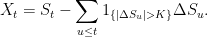
Proof: Fixing K > 0, decompose S as,
 |
where Y, Z are pure jump processes consisting of the jumps larger than K and less than –K respectively.
 |
First, look at X. As it is a Lévy process with bounded jumps (by K), it is square integrable, and by independent increments, both 𝔼[Xt] and the variance Var(Xt) are linear in time,
![\displaystyle {\mathbb E}[X_t]=at,\ {\rm Var}(X_t)=bt.](https://s0.wp.com/latex.php?latex=%5Cdisplaystyle+%7B%5Cmathbb+E%7D%5BX_t%5D%3Dat%2C%5C+%7B%5Crm+Var%7D%28X_t%29%3Dbt.+&bg=ffffff&fg=000000&s=0&c=20201002) |
Applying Doob’s inequality to the martingale Xt – at,
![\displaystyle {\mathbb E}\left[\sup_{s\le t}X_s^2\right]\le {\mathbb E}[2\sup_{s\le t}(X_s-as)^2]+2a^2t^2\le 8bt+2a^2t^2](https://s0.wp.com/latex.php?latex=%5Cdisplaystyle+%7B%5Cmathbb+E%7D%5Cleft%5B%5Csup_%7Bs%5Cle+t%7DX_s%5E2%5Cright%5D%5Cle+%7B%5Cmathbb+E%7D%5B2%5Csup_%7Bs%5Cle+t%7D%28X_s-as%29%5E2%5D%2B2a%5E2t%5E2%5Cle+8bt%2B2a%5E2t%5E2+&bg=ffffff&fg=000000&s=0&c=20201002) |
and, hence,
![\displaystyle {\mathbb E}\left[\sup_{s\le t}X_s\right]\le \sqrt{8bt+2a^2t^2}](https://s0.wp.com/latex.php?latex=%5Cdisplaystyle+%7B%5Cmathbb+E%7D%5Cleft%5B%5Csup_%7Bs%5Cle+t%7DX_s%5Cright%5D%5Cle+%5Csqrt%7B8bt%2B2a%5E2t%5E2%7D+&bg=ffffff&fg=000000&s=0&c=20201002) |
which is bounded by a multiple of √t over each finite time interval.
Next, look at the nonnegative term Yt. If we suppose that St+ is integrable for a single t > 0 then, since Yt – Zt = St–Xt is integrable and Y, Z are independent, it follows that Yt is integrable. By independent increments, Yt is integrable for all t and 𝔼[Yt] = ct for some nonnegative constant c. Hence,
![\displaystyle {\mathbb E}[R_t]\le{\mathbb E}\left[\sup_{s\le t}(Y_s+Z_s)\right]\le\sqrt{8bt+2a^2t^2}+ct](https://s0.wp.com/latex.php?latex=%5Cdisplaystyle+%7B%5Cmathbb+E%7D%5BR_t%5D%5Cle%7B%5Cmathbb+E%7D%5Cleft%5B%5Csup_%7Bs%5Cle+t%7D%28Y_s%2BZ_s%29%5Cright%5D%5Cle%5Csqrt%7B8bt%2B2a%5E2t%5E2%7D%2Bct+&bg=ffffff&fg=000000&s=0&c=20201002) |
which is bounded by a multiple of √t over bounded time intervals.
Finally, as Lévy processes are continuous in probability, if tn → t then Stn → St in probability. As St+ is bounded by the increasing integrable process Rt, dominated convergence says that 𝔼[S+tn] → 𝔼[St+] which, therefore, is continuous in t. ⬜
The following bound was required for the proof of theorem 9.
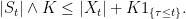
Lemma 12 For any fixed K > 0, 𝔼[|St| ∧ K] is bounded by a multiple of √t.
Proof: First, f(t) = 𝔼[|St| ∧ K] is bounded by K and, hence, is bounded by a multiple of √t away from 0. So, it is sufficient to show that f(t) = O(√t) as t → 0. Then, as in the proof of lemma 11, we strip out the jumps of S which are larger than K in absolute value,
 |
As the jumps of St greater than K in absolute value arrive according to a Poisson process of some finite rate λ ≥ 0, the first time τ at which such a jump occurs has the exponential distribution with rate parameter λ. Taking expectations of the inequality
 |
we obtain
![\displaystyle f(t)\le{\mathbb E}[\lvert X_t\rvert]+K(1-e^{-\lambda t}).](https://s0.wp.com/latex.php?latex=%5Cdisplaystyle+f%28t%29%5Cle%7B%5Cmathbb+E%7D%5B%5Clvert+X_t%5Crvert%5D%2BK%281-e%5E%7B-%5Clambda+t%7D%29.+&bg=ffffff&fg=000000&s=0&c=20201002) |
As in the proof of lemma 11, 𝔼[|Xt|] = O(√t), so the right hand side of the above inequality is bounded by a multiple of √t as t → 0. ⬜
Proof of Spitzer’s Formula
I give a proof of Spitzer’s formula, based on the treatment in the 1958 paper Spitzer’s formula: A short proof by J.G. Wendell. It is actually rather surprising how such a seemingly complicated result drops almost effortlessly out of some very basic algebra. While this section might look quite long at first glance, most of it consists of simply defining the algebraic structures and elementary manipulations. After that, there is very little real work. The real meat that seems to contribute to the final result is the algebraic properties of the projection operator P stated in lemma 13 below. This lemma is still rather simple though.
Use M to denote the finite complex Borel measures on ℝ2, which is a vector space over ℂ. The idea is that the distribution of (Rn, Sn) is in M and needs to be constructed. Note that we construct Sn+1 by adding independent random variable Xn+1 to Sn and then obtain Rn+1 by taking the maximum of this with Rn,
 |
This can be represented by a pair of linear operators on M , which I denote by F and P respectively. If (R, S) are random variables with probability distribution μ ∈ M then Fμ represents the distribution of (R, S + X) where X has the random walk increment distribution (i.e., same as Xk) and is independent of (R, S). Also, Pν represents the distribution of (R ∨ S, S). That is, they are linear maps M → M satisfying
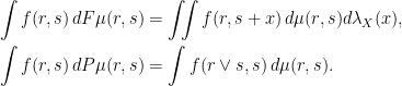 |
for μ ∈ M and bounded measurable f: ℝ2 → ℂ, where λX denotes the distribution of X. By construction, if μ is the distribution of (Rn, Sn) then Fμ is the distribution of (Rn, Sn+1) and PFμ is the distribution of (Rn+1, Sn+1). That is,
 |
where γn ∈ M is the distribution of (Rn, Sn).
Use δ ∈ M to denote the ‘Dirac delta’ distribution on ℝ2 under which (R, S) satisfy R = S = 0 almost surely. Then, γ0 = δ and, iteratively applying the equation above gives
 |
(13) |
Next we promote M to an algebra over ℂ by using convolution as the multiplication operator. If μ, ν ∈ M are distributions of (R1, S1) and (R2, S2) respectively, and these are independent, then μν is the distribution of (R1 + R2, S1 + S2). Explicitly
 |
for bounded measurable f: ℝ2 → ℂ. This is a commutative ring with identity δ, δμ = μδ = μ.
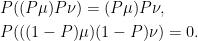
It should be clear from the definition that P is a projection, P2 = P. However, it also satisfies the following properties which will be instrumental in proving Spitzer’s formula. These are equivalent saying that PM and (1 - P)M are subalgebras.
Lemma 13 The operator P satisfies the following identities for any μ, ν ∈ M ,
- if Pμ = μ and Pν = ν then P(μν) = μν.
- if Pμ = Pν = 0 then P(μν) = 0.
Proof: The statements are equivalent to the identities
 |
By linearity it is sufficient to prove these for probability measures, so suppose that (R1, S1) and (R2, S2) are independent with distributions μ and ν respectively. From the definitions
 |
has distribution (Pμ)Pν. As R ≥ S, applying P to this has no effect, proving the first identity. The second identity can be rearranged as
 |
(14) |
The terms on the left hand side are the distributions of (R, S1 + S2) with R equal to
 |
respectively. For the right hand side, R is equal to
 |
respectively. On {R1 ≥ S1} these are the same pairs of values, so that P(μν) = P((Pμ)ν) and (Pμ)Pν = P(μPν). On {R2 ≥ S2}, they are the same pairs but in different order, so P(μν) = P(μPν) and (Pμ)Pν = P((Pμ)ν). On the remaining case with R1 < S1 and R2 < S2 they all reduce to R = S1 + S2. So, in all cases, (14) holds. ⬜
Curiously, the paper by Wendell does not prove a version of lemma 13. Instead, it merely states that PM and (1 - P)M are subalgebras as if it is an obvious fact. As these properties appear to be the central facts on which the proof is built, and are not obvious to me, I included the statement and proof.
Now, consider the space M [[t]] of power series over M in indeterminate t. This consists of series
 |
for coefficients μk lying in M . Performing addition and multiplication term-by-term makes this into an algebra, to which the operators F and P can be extended by applying to the the coefficients.
Equation (13) can be expressed by a simple formula for the generating function of the sequence γn.
Lemma 14 The operator 1 – tPF on M [[t]] is invertible and
(15)

Proof: It is easily checked that the operator 1 – tPF has inverse
 |
As for a standard geometric series, just multiply by 1 – tPF and note that all powers of t cancel leaving only 1. Applying to δ directly gives the left hand side of (15) by substituting in (13). ⬜
Any function f(z) given by a power series with complex coefficients can be defined on tM [[t]]. Here, we just need exponentials and logarithms,
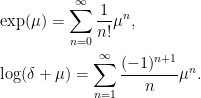 |
These are well-defined as long as μ ∈ M [[t]] is a multiple of t, so that nonzero coefficients of any fixed power of t only occur in finitely terms on the right. They satisfy the usual identities
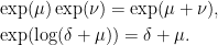 |
This can be checked by expanding and comparing powers of μ and ν, which we know must verify the correct identities since they hold over the complex numbers.
Now let χ ∈ M be the distribution of (0, X),
![\displaystyle \int f(r,s)\,d\chi(r,s)=\int f(0,x)\,d\lambda_X(x)={\mathbb E}[f(0,X)].](https://s0.wp.com/latex.php?latex=%5Cdisplaystyle+%5Cint+f%28r%2Cs%29%5C%2Cd%5Cchi%28r%2Cs%29%3D%5Cint+f%280%2Cx%29%5C%2Cd%5Clambda_X%28x%29%3D%7B%5Cmathbb+E%7D%5Bf%280%2CX%29%5D.+&bg=ffffff&fg=000000&s=0&c=20201002) |
With this definition, the operator F is the same as multiplying by χ.
Proving the following formula for the generating function of γn is now just a matter of simple algebra combined with the properties of P stated in lemma 13. This is essentially an alternative statement of Spitzer’s theorem. In many ways, I actually prefer the formulation given below over the version of Spitzer’s theorem stated in 1 and 2 above, since it directly works with distributions rather than characteristic functions.
Theorem 15
(16)

Proof: Letting γ∗ denote the right hand side of (16), this is of the form exp(μ) where Pμ = μ. Expanding it out gives a sum of multiples of powers of μ which, by lemma 13, are invariant under applying P. Hence, Pγ∗ = γ∗.
Now,
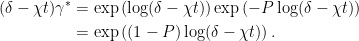 |
The right hand side is of the form exp(μ) for Pμ = 0. Expanding this out gives δ + ν where ν is a sum of multiples of positive powers of μ. It follows from lemma 13 that Pν = 0. Hence,
 |
We obtain
 |
Lemma 14 gives
 |
as required. ⬜
We finish off by expressing the result in terms of characteristic functions to obtain Spitzer’s theorem as stated at the top of the post.
Proof of theorems 1 and 2: As the two statements are equivalent under a change of variables, we just need to prove theorem 2. Fixing reals α, β, define f: ℝ2 → ℂ by f(r, s) = exp(iαr + iβs). Writing μ(f) for the integral of f with respect to measure μ,
![\displaystyle \begin{aligned} &\gamma_n(f)={\mathbb E}\left[e^{i\alpha R_n+i\beta S_n}\right]\equiv\tilde\phi_n,\\ &(P\chi^n)(f)={\mathbb E}\left[e^{i\alpha S_n^++i\beta S_n}\right]\equiv\tilde w_n. \end{aligned}](https://s0.wp.com/latex.php?latex=%5Cdisplaystyle+%5Cbegin%7Baligned%7D+%26%5Cgamma_n%28f%29%3D%7B%5Cmathbb+E%7D%5Cleft%5Be%5E%7Bi%5Calpha+R_n%2Bi%5Cbeta+S_n%7D%5Cright%5D%5Cequiv%5Ctilde%5Cphi_n%2C%5C%5C+%26%28P%5Cchi%5En%29%28f%29%3D%7B%5Cmathbb+E%7D%5Cleft%5Be%5E%7Bi%5Calpha+S_n%5E%2B%2Bi%5Cbeta+S_n%7D%5Cright%5D%5Cequiv%5Ctilde+w_n.+%5Cend%7Baligned%7D+&bg=ffffff&fg=000000&s=0&c=20201002) |
The fact that the characteristic function of the sum of independent random variables is the product of their characteristic functions means that (μν)(f) = μ(f)ν(f) for μ, ν ∈ M or, equivalently, integration of f is a homomorphism from M to ℂ. Applying termwise, this gives a homomorphism from M [[t]] to ℂ[[t]]. Applying (16) to f gives the result.
 |
⬜

Can this also be applied to the distribution of the maximum distance from the origin? I.e. $|R_n|$ in your notation.
Well, R_n is nonnegative in my notation, so I don’t think you mean |R_n|. I assume you mean, max_{k <= n}|S_k|. Then, no. The absolute maximum is rather different. Compare the absolute maximum of Brownian motion which requires infinite sum, with the much simpler (non-absolute) maximum.
1
1*1
1*949*944*0
1+954-949-5
1*911*906*0
1+916-911-5
1*887*882*0
1+892-887-5
1′”
@@LthMx
There is a beautiful theory of convex minorants of random walk and Levy processes due to Pitman and el., which extends the idea of Spitzer’s lemma: one can recover the Spitzer’s lemma by considering the faces of convex minorants with negative slopes. See e.g. https://arxiv.org/abs/1102.0818
1
1*1
1-1; waitfor delay ‘0:0:15’ —
1-1); waitfor delay ‘0:0:15’ —
1-1 waitfor delay ‘0:0:15’ —
1′”