Levy Process – Almost Sure

Spitzer’s formula is a remarkable result giving the precise joint distribution of the maximum and terminal value of a random walk in terms of the marginal distributions of the process. I have already covered the use of the reflection principle to describe the maximum of Brownian motion, and the same technique can be used for simple symmetric random walks which have a step size of ±1. What is remarkable about Spitzer’s formula is that it applies to random walks with any step distribution.

We consider partial sums

$\displaystyle S_n=\sum_{k=1}^n X_k$

for an independent identically distributed (IID) sequence of real-valued random variables X₁, X₂, …. This ranges over index n = 0, 1, … starting at S₀ = 0 and has running maximum

$\displaystyle R_n=\max_{k=0,1,\ldots,n}S_k.$

Spitzer’s theorem is typically stated in terms of characteristic functions, giving the distributions of (R_n, S_n) in terms of the distributions of the positive and negative parts, S_n⁺ and S_n^–, of the random walk.

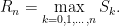
Theorem 1 (Spitzer) For α, β ∈ ℝ,

$\displaystyle \sum_{n=0}^\infty \phi_n(\alpha,\beta)t^n=\exp\left(\sum_{n=1}^\infty w_n(\alpha,\beta)\frac{t^n}{n}\right)$ (1)

where ϕ_n, w_n are the characteristic functions

$\displaystyle \begin{aligned} \phi_n(\alpha,\beta)&={\mathbb E}\left[e^{i\alpha R_n+i\beta(R_n-S_n)}\right],\\ w_n(\alpha,\beta)&={\mathbb E}\left[e^{i\alpha S_n^++i\beta S_n^-}\right]\\ &={\mathbb E}\left[e^{i\alpha S_n^+}\right]+{\mathbb E}\left[e^{i\beta S_n^-}\right]-1. \end{aligned}$

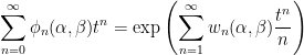
As characteristic functions are bounded by 1, the infinite sums in (1) converge for |t|< 1. However, convergence is not really necessary to interpret this formula, since both sides can be considered as formal power series in indeterminate t, with equality meaning that coefficients of powers of t are equated. Comparing powers of t gives

$\displaystyle \begin{aligned} \phi_1&=w_1,\\ \phi_2&=\frac{w_1^2}2+\frac{w_2}2,\\ \phi_3&=\frac{w_1^3}6+\frac{w_1w_2}2+\frac{w_3}3, \end{aligned}$

(2)

and so on.

Spitzer’s theorem in the form above describes the joint distribution of the nonnegative random variables (R_n, R_n - S_n) in terms of the nonnegative variables (S_n⁺, S_n^–). While this does have a nice symmetry, it is often more convenient to look at the distribution of (R_n, S_n) in terms of (S_n⁺, S_n), which is achieved by replacing α with α + β and β with –β in (1). This gives a slightly different, but equivalent, version of the theorem.

Theorem 2 (Spitzer) For α, β ∈ ℝ,

$\displaystyle \sum_{n=0}^\infty \tilde\phi_n(\alpha,\beta)t^n=\exp\left(\sum_{n=1}^\infty \tilde w_n(\alpha,\beta)\frac{t^n}{n}\right)$ (3)

where ϕ̃_n, w̃_n are the characteristic functions

$\displaystyle \begin{aligned} \tilde\phi_n(\alpha,\beta)&={\mathbb E}\left[e^{i\alpha R_n+i\beta S_n}\right],\\ \tilde w_n(\alpha,\beta)&={\mathbb E}\left[e^{i\alpha S_n^++i\beta S_n}\right]. \end{aligned}$

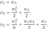
Taking β = 0 in either (1) or (3) gives the distribution of R_n in terms of S_n⁺,

$\displaystyle \sum_{n=0}^\infty {\mathbb E}\left[e^{i\alpha R_n}\right]t^n=\exp\left(\sum_{n=1}^\infty {\mathbb E}\left[e^{i\alpha S_n^+}\right]\frac{t^n}n\right)$

(4)

I will give a proof of Spitzer’s theorem below. First, though, let’s look at some consequences, starting with the following strikingly simple result for the expected maximum of a random walk.

Corollary 3 For each n ≥ 0,

$\displaystyle {\mathbb E}[R_n]=\sum_{k=1}^n\frac1k{\mathbb E}[S_k^+].$ (5)

Proof: As R_n ≥ S₁⁺ = X₁⁺, if X_k⁺ have infinite mean then both sides of (5) are infinite. On the other hand, if X_k⁺ have finite mean then so do S_n⁺ and R_n. Using the fact that the derivative of the characteristic function of an integrable random variable at 0 is just i times its expected value, compute the derivative of (4) at α = 0,

$\displaystyle \begin{aligned} \sum_{n=0}^\infty i{\mathbb E}[R_n]t^n &=\exp\left(\sum_{n=1}^\infty \frac{t^n}n\right)\sum_{n=1}^\infty i{\mathbb E}[S_n^+]\frac{t^n}n\\ &=\exp\left(-\log(1-t)\right)\sum_{n=1}^\infty i{\mathbb E}[S_n^+]\frac{t^n}n\\ &=(1-t)^{-1}\sum_{n=1}^\infty i{\mathbb E}[S_n^+]\frac{t^n}n\\ &=(1+t+t^2+\cdots)\sum_{n=1}^\infty i{\mathbb E}[S_n^+]\frac{t^n}n. \end{aligned}$

Equating powers of t gives the result. ⬜

The expression for the distribution of R_n in terms of S_n⁺ might not be entirely intuitive at first glance. Sure, it describes the characteristic functions and, hence, determines the distribution. However, we can describe it more explicitly. As suggested by the evaluation of the first few terms in (2), each ϕ_n is a convex combination of products of the w_n. As is well known, the characteristic function of the sum of random variables is equal to the product of their characteristic functions. Also, if we select a random variable at random from a finite set, then its characteristic function is a convex combination of those of the individual variables with coefficients corresponding to the probabilities in the random choice. So, (3) expresses the distribution of (R_n, S_n) as a random choice of sums of independent copies of (S_k⁺, S_k).

In fact, expressions such as (1,3) are common in many branches of maths, such as zeta functions associated with curves over finite fields. We have a power series which can be expressed in two different ways,

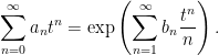$\displaystyle \sum_{n=0}^\infty a_nt^n = \exp\left(\sum_{n=1}^\infty b_n\frac{t^n}n\right).$

The left hand side is the generating function of the sequence a_n. The right hand side is a kind of zeta function associated with the sequence b_n, and is sometimes referred to as the combinatorial zeta function. The logarithmic derivative gives Σ_nb_nt^n-1, which is the generating function of b_n+1. Continue reading “Spitzer’s Formula” →

	Anonymous on About
	Anonymous on About
	Anonymous on The Stochastic Integral
	Anonymous on Bessel Processes
	Anonymous on Bessel Processes
	Stat Prof on Pathwise Regularity of Optiona…
	Yang Chu on Spitzer’s Formula
	Anonymous on About
	Anonymous on Continuous Processes with Inde…
	Anonymous on Continuous Processes with Inde…