Spitzer’s formula is a remarkable result giving the precise joint distribution of the maximum and terminal value of a random walk in terms of the marginal distributions of the process. I have already covered the use of the reflection principle to describe the maximum of Brownian motion, and the same technique can be used for simple symmetric random walks which have a step size of ±1. What is remarkable about Spitzer’s formula is that it applies to random walks with any step distribution.
We consider partial sums
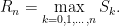
for an independent identically distributed (IID) sequence of real-valued random variables X1, X2, …. This ranges over index n = 0, 1, … starting at S0 = 0 and has running maximum
Spitzer’s theorem is typically stated in terms of characteristic functions, giving the distributions of (Rn, Sn) in terms of the distributions of the positive and negative parts, Sn+ and Sn–, of the random walk.
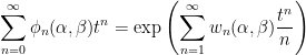
Theorem 1 (Spitzer) For α, β ∈ ℝ,
(1)
where ϕn, wn are the characteristic functions
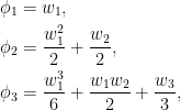
As characteristic functions are bounded by 1, the infinite sums in (1) converge for |t|< 1. However, convergence is not really necessary to interpret this formula, since both sides can be considered as formal power series in indeterminate t, with equality meaning that coefficients of powers of t are equated. Comparing powers of t gives
(2)
and so on.
Spitzer’s theorem in the form above describes the joint distribution of the nonnegative random variables (Rn, Rn - Sn) in terms of the nonnegative variables (Sn+, Sn–). While this does have a nice symmetry, it is often more convenient to look at the distribution of (Rn, Sn) in terms of (Sn+, Sn), which is achieved by replacing α with α + β and β with –β in (1). This gives a slightly different, but equivalent, version of the theorem.
Theorem 2 (Spitzer) For α, β ∈ ℝ,
(3)
where ϕ̃n, w̃n are the characteristic functions
Taking β = 0 in either (1) or (3) gives the distribution of Rn in terms of Sn+,
(4)
I will give a proof of Spitzer’s theorem below. First, though, let’s look at some consequences, starting with the following strikingly simple result for the expected maximum of a random walk.
Corollary 3 For each n ≥ 0,
(5)
Proof: As Rn ≥ S1+ = X1+, if Xk+ have infinite mean then both sides of (5) are infinite. On the other hand, if Xk+ have finite mean then so do Sn+ and Rn. Using the fact that the derivative of the characteristic function of an integrable random variable at 0 is just i times its expected value, compute the derivative of (4) at α = 0,
Equating powers of t gives the result. ⬜
The expression for the distribution of Rn in terms of Sn+ might not be entirely intuitive at first glance. Sure, it describes the characteristic functions and, hence, determines the distribution. However, we can describe it more explicitly. As suggested by the evaluation of the first few terms in (2), each ϕn is a convex combination of products of the wn. As is well known, the characteristic function of the sum of random variables is equal to the product of their characteristic functions. Also, if we select a random variable at random from a finite set, then its characteristic function is a convex combination of those of the individual variables with coefficients corresponding to the probabilities in the random choice. So, (3) expresses the distribution of (Rn, Sn) as a random choice of sums of independent copies of (Sk+, Sk).
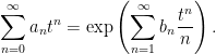
In fact, expressions such as (1,3) are common in many branches of maths, such as zeta functions associated with curves over finite fields. We have a power series which can be expressed in two different ways,
The left hand side is the generating function of the sequence an. The right hand side is a kind of zeta function associated with the sequence bn, and is sometimes referred to as the combinatorial zeta function. The logarithmic derivative gives Σnbntn-1, which is the generating function of bn+1. Continue reading “Spitzer’s Formula”→
In a 1986 article of The American Mathematical Monthly written by Richard Guy, the following question was asked, and attributed to Bogusłav Tomaszewski: Consider n real numbers a1, …, an such that Σiai2 = 1. Of the 2n expressions |±a1±⋯±an|,
can there be more with value > 1 than with value ≤ 1?
A cursory attempt to find such real numbers ai where more of the absolute signed sums have value > 1 than have value ≤ 1 should be enough to convince you that it is, in fact, impossible. The answer was therefore expected to be no, it is not possible. This has claim since been known as Tomaszewski’s conjecture, and there have been many proofs of weaker versions over the years until, finally, in 2020, it was proved by Keller and Klein in the paper Proof of Tomaszewski’s Conjecture on Randomly Signed Sums.
where X1, …, Xn are independent ‘random signs’. That is, they have the Rademacher distribution ℙ(Xi = 1) = ℙ(Xi = -1) = 1/2. Then, Z has variance Σiai2 and each of the 2n values ±a1±⋯±an occurs with equal probability. So, Tomaszewski’s conjecture is the statement that
(2)
for unit variance Rademacher sums Z. It is usually stated in the equivalent, but more convenient form
(3)
I will discuss Tomaszewski’s conjecture and the ideas central to the proof given by Keller and Klein. I will not give a full derivation here. That would get very tedious, as evidenced both by the length of the quoted paper and by its use of computer assistance. However, I will prove the ‘difficult’ cases, which makes use of the tricks essential to Keller and Klein’s proof, with all remaining cases being, in theory, provable by brute force. In particular, I give a reformulation of the inductive stopping time argument that they used. This is a very ingenious trick that was introduced by Keller and Klein, and describing this is one of the main motivations for this post. Another technique also used in the proof is based on the reflection principle, in addition to some tricks discussed in the earlier post on Rademacher concentration inequalities.
To get a feel for Rademacher sums, some simple examples are shown in figure 1. I use the notation a = (a1, …, an) to represent the sequence with first n terms given by ai, and any remaining terms equal to zero. The plots show the successive partial sums for each sequence of values of the random signs (X1, X2, …), with the dashed lines marking the ±1 levels.
Figure 1: Example Rademacher sums
The examples demonstrate that ℙ(|Z| ≤ 1) can achieve the bound of 1/2 in some cases, and be strictly more in others. The top-left and bottom-right plots show that, for certain coefficients, |Z| has a positive probability of being exactly equal to 1 and, furthermore, the claimed bound fails for ℙ(|Z|< 1). So, the inequality is optimal in a couple of ways. These examples concern a small number of nonzero coefficients. In the other extreme, for a large number of small coefficients, the central limit theorem says that Z is approximately a standard normal and ℙ(|Z| ≤ 1) is close to Φ(1) – Φ(-1) ≈ 0.68. Continue reading “Tomaszewski’s Conjecture”→
Concentration inequalities place lower bounds on the probability of a random variable being close to a given value. Typically, they will state something along the lines that a variable Z is within a distance x of value μ with probability at least p,
(1)
Although such statements can be made in more general topological spaces, I only consider real valued random variables here. Clearly, (1) is the same as saying that Z is greater than distance x from μ with probability no more than q = 1 – p. We can express concentration inequalities either way round, depending on what is convenient. Also, the inequality signs in expressions such as (1) may or may not be strict. A very simple example is Markov’s inequality,
In the other direction, we also encounter anti-concentration inequalities, which place lower bounds on on the probability of a random variable being at least some distance from a specified value, so take the form
While the examples given above of the Markov and Paley-Zygmund inequalities are very general, applying whenever the required moments exist, they are also rather weak. For restricted classes of random variables much stronger bounds can often be obtained. Here, I will be concerned with optimal concentration and anti-concentration bounds for Rademacher sums. Recall that these are of the form
for IID random variables X = (X1, X2, …) with the Rademacher distribution, ℙ(Xn = 1) = ℙ(Xn = -1) = 1/2, and a = (a1, a2, …) is a square-summable sequence. This sum converges to a limit with zero mean and variance
I discussed such sums at length in the posts on Rademacher series and the Khintchine inequality, and have been planning on making this follow-up post ever since. In fact, the L0 Khintchine inequality was effectively the same thing as an anti-concentration bound. It was far from optimal as presented there, and relied on the rather inefficient Paley-Zygmund inequality for the proof. Recently, though, a paper was posted on arXiv claiming to confirm conjectured optimal anti-concentration bounds which I had previous mentioned on mathoverflow. See Tight lower bounds for anti-concentration of Rademacher sums and Tomaszewski’s counterpart problem by Lawrence Hollom and Julien Portier.
While the form of the tight Rademacher concentration and anti-concentration bounds may seem surprising at first, being piecewise constant and jumping between rather arbitrary looking rational values at seemingly arbitrary points, I will explain why this is so. It is actually rather interesting and has been a source of conjectures over the past few decades, some of which have now been proved and some which remain open. Actually, as I will explain, many tight bounds can be proven in principle by direct computation, although it would be rather numerically intensive to perform in practice. In fact, some recent results — including those of Hollom and Portier mentioned above — were solved with the aid of a computer to perform the numerical legwork.
Anti-Concentration Bounds
Figure 1: Optimal anti-concentration bounds
For a Rademacher sum Z of unit variance, recall from the post on the Khintchine inequality that the anti-concentration bound
(3)
holds for all non-negative x ≤ 1. This followed from Payley-Zygmund together with the simple Khintchine inequality 𝔼[Z2] ≤ 3. However, this is sub-optimal and is especially bad in the limit as x increases to 1 where the bound tends to zero whereas, as we will see, the optimal bound remains strictly positive.
In the other direction if, for positive integer n, we choose coefficients a ∈ ℓ2 with ak = 1/√n for k ≤ n and zero elsewhere then, by the central limit theorem, Z = a·X tends to a standard normal distribution. as n becomes large. Hence
where Φ is the cumulative normal distribution function. So, any anti-concentration bound must be no more than this.
The optimal anti-concentration bounds have been open conjectures for a while, but are now proved and described by theorem 1 below, as plotted in figure 1. They are given by a piecewise constant function and, as clear from the plot, lie strictly between the simple Paley-Zymund bound and Gaussian probabilities.
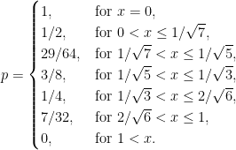
Theorem 1 The optimal lower bound p for the inequality ℙ(|Z| ≥ x) ≥ p for Rademacher sums Z of unit variance is,
At first sight, this result might seem a little strange. Why do the optimal bounds take this discrete set of values, and why does it jump at these arbitrary seeming values of x? To answer that, consider the distribution of a Rademacher sum. When all coefficients are small it approximates a standard normal and the anti-concentration probabilities approach those indicated by the ‘Gaussian bound’ in figure 1. However, these are not optimal, and the minimal probabilities are obtained at the opposite extreme with a small number n of relatively large coefficients and the remaining being zero. In this case, the distribution is finite with probabilities being multiples of 2–n, and the bound jumps when x passes through the discrete levels.
The values of a ∈ ℓ2 for which the stated bounds are achieved are not hard to find. For convenience, I use (a1, a2, …, an) to represent the sequence starting with the stated values and remaining terms being zero, ak = 0 for k > n. Also, if c is a numeral than ck will denote repeating this value k times.
Lemma 2 The optimal lower bound stated by theorem 1 for Rademacher sum Z = a·X is achieved with
This is straightforward to verify by simply counting the number of sign values of (X1, |, Xn) for which |a·X| ≥ x and multiplying by 2–n. It does however show that it is impossible to do better than theorem 1 so that, if the bounds hold, they must be optimal. Also, as ℙ(|Z| ≥ x) is decreasing in x, to establish the result it is sufficient to show that the bounds hold at the values of x where it jumps. This reduces theorem 1 to the following finite set of inequalities.
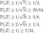
Theorem 3 A Rademacher sum Z of unit variance satisfies,
The last of these has been an open conjecture for years since it was mentioned in a 1996 paper by Oleszkiewicz. I asked about the first one in a 2021 mathoverflow question, and also mentioned the finite set of values x at which the optimal bound jumps, hinting at the full set of inequalities, which was the desired goal. Finally, in 2023, a preprint appeared on arXiv claiming to prove all of these. While I have not completely verified the proof and the computer programs used myself, it does look likely to be correct.
Although the bounds given above are all for anti-concentration about 0, a simple trick shows that they will also hold about any real value.
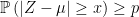
Lemma 4 Suppose that the inequality ℙ(|Z| ≥ x) ≥ p holds for all Rademacher sums Z of unit variance. Then the anti-concentration bound
also holds about every value μ.
Proof: If Z = a·X and, independently, Y is a Rademacher random variable, then Z + μY is a Rademacher sum of variance 1 + μ2. This follows from the fact that it has the same distribution as b·X where b = (μ, a1, a2, …). So,
By symmetry of the distribution of Z, both probabilities on the right are equal giving,
implying the result. ⬜
You have probably noted already, that all of the coefficients described in lemma 2 are of the form (1n)/√n. That is, they are a finite a sequence of equal values with the remaining terms being zero. In fact, it has been conjectured that all optimal concentration and anti-concentration bounds (about 0) for Rademacher sums can be attained in this way. This is attributed to Edelman dating back to private communications in 1991. If true, it would turn the process of finding and proving such optimal bounds into a straightforward calculation but, unfortunately, in 2012, the conjecture was shown to be false by Pinelis for some concentration inequalities.
Before moving on, let’s mention how such bounds can be discovered in the first place. Running a computer simulation for randomly chosen finite sequences of coefficients very quickly converges on the optimal values. As soon as we randomly select values close to those given by lemma 2, we obtain the exact bounds and any further simulations only serve to verify that these hold. Running additional simulations with coefficients chosen randomly in the neighbourhood of points where the bound is attained, and near certain ‘critical’ values where the bound looks close to being broken, further strengthens the belief that they are indeed optimal. At least, this is how I originally found them before asking the mathoverflow question, although this is still far from a proof.
Probability and measure theory relies on the concept of measurable sets. On the real numbers ℝ, in particular, there are several different sigma-algebras which are commonly used, and a set is said to be measurable if it lies in the one under consideration. Probabilities and measures are only defined for events lying in a specific sigma-algebra, so it is essential to know if sets are measurable. Fortunately, most simply constructed events will indeed be measurable, but this is not always the case. In fact, once we start working with more complex setups, such as continuous-time stochastic processes observed at random times, non-measurable sets occur more commonly than might be expected. To avoid such issues, it is usual to enlarge the underlying sigma-algebra defining a probability space as much as possible.
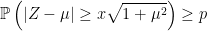
The Borel sets form the smallest sigma-algebra containing the open sets or, equivalently, containing all intervals. This is denoted as , which I will also shorten to . An explicit construction of a non-Borel set was given by Lusin in 1927. Every irrational real number can be expressed uniquely as a continued fraction
where a0 is an integer and ai are positive integers for i ≥ 1. Lusin considered the set of irrationals whose continued fraction coefficients contain a subsequence ak1, ak2, … such that each term is a divisor of the subsequent term.
Other examples can be given along similar lines to Lusin’s. Every real number has a binary expansion
where a0 is an integer and ai is in {0, 1} for each i ≥ 1. Consider the set of reals having a binary expansion for which there is an infinite sequence of positive integers k1, k2, …, each term strictly dividing the next, such that aki = 1. I will give proofs that these examples are non-Borel in this post.
There is a general method of enlarging sigma-algebras known as the completion. Consider a measure μ defined on a measurable space consisting of sigma-algebra on set X. The completion consists of all subsets S ⊆ X which can be sandwiched between sets in whose difference has zero measure. That is, A ⊆ S ⊆ B for with μ(B ∖ A) = 0. It can be shown that is a sigma-algebra containing , and μ uniquely extends to a measure on this by taking μ(S) = μ(A) = μ(B) for S, A, B as above.
The Lebesgue measure λ is uniquely defined on the Borel sets by specifiying its value on intervals as λ((a, b)) = b – a. The completion is the Lebesgue sigma-algebra, which I will denote by . Usually, when saying that a subset of the reals is measurable without further qualification, it is understood to mean that it is in . The non-Borel set constructed by Lusin can be shown to be measurable (in fact, its complement has zero Lebesgue measure).
While the Lebesgue measure extends uniquely to , this is not true for for all measures defined on the Borel sigma-algebra. In particular, it will not be true for singular measures, which assign a positive value to some Lebesgue-null sets. An example is the uniform probability measure (or, Haar measure) on the Cantor middle-thirds setC. This has zero Lebesgue measure, so every subset of C is in , but the uniform measure on C cannot be extended uniquely to all subsets. For this reason, universal completions are often used. For a measurable space , the universal completion consists of the subsets of X which lie in the completion of with respect to every possible sigma-finite measure.
The intersection is taken over all sigma-finite measures μ on . It is enough to take the intersection over finite or, even, probability measures, since every sigma-finite measure is equivalent to such. The universal completion is a bit tricky to understand in an explicit way but, by construction, all sigma-finite measures on a sigma-algebra extend uniquely to its universal completion. It can be shown that Lusin’s example of a non-Borel set does lie in the universal completion .
Finally, the power set consisting of all subsets of a set X is a sigma-algebra. For uncountable sets such as the reals, this is often too large to be of use and measures cannot be extended in any unique way. However, we have four common sigma-algebras of the real numbers,
(1)
In this post, I show that each of these inclusions is strict. That is, there are subsets of the reals which are not Lebesgue measurable, there are Lebesgue sets which are not in the universal completion , and there are sets in which are not Borel. Lusin’s construction is an example of the latter. The strictness of the other two inclusions does depend crucially on the axiom of choice so, unlike Lusin’s set, the examples demonstrating that these are strict are not explicit. Continue reading “Non-Measurable Sets”→
According to Kolmogorov’s axioms, to define a probability space we start with a set Ω and an event space consisting of a sigma-algebra F on Ω. A probability measure ℙ on this gives the probability space (Ω, F , ℙ), on which we can define random variables as measurable maps from Ω to the reals or other measurable space.
However, it is common practice to suppress explicit mention of the underlying sample spaceΩ. The values of a random variable X: Ω → ℝ are simply written as X, rather than X(ω) for ω ∈ Ω. It is intuitively thought of as a real number which happens to be random, rather than a function. For one thing, we usually do not really care what the sample space is and, instead, only care about events and their probabilities, and about random variables and their expectations. This philosophy has some benefits. Frequently, when performing constructions, it can be useful to introduce new supplementary random variables to work with. It may be necessary to enlarge the sample space and add new events to the sigma-algebra to accommodate these. If the underlying space is not set in stone then this is straightforward to do, and we can continue to work with these new variables as if they were always there from the start.
Definition 1 An extension π of a probability space (Ω, F , ℙ) to a new space (Ω′, F ′, ℙ′),
is a probability preserving measurable map π: Ω′ → Ω. That is, ℙ′(π-1E) = ℙ(E) for events E ∈ F .
By construction, events E ∈ F pull back to events π-1E ∈ F ′ with the same probabilities. Random variables X defined on (Ω, F , ℙ) lift to variables π∗X with the same distribution defined on (Ω′, F ′, ℙ′), given by π∗X(ω) ≡ X(π(ω)). I will use the notation X∗ in place of π∗X for brevity although, in applications, it is common to reuse the same symbol X and simply note that we are now working with respect to an enlarged the probability space if necessary.
The extension can be thought of in two steps. First, the enlargement of the sample space, π: Ω′ → Ω on which we induce the sigma algebra π∗F consisting of events π-1E for E ∈ F , and the measure ℙ′(π-1E) = ℙ(E). This is essentially a no-op, since events and random variables on the initial space are in one-to-one correspondence with those on the enlarged space (at least, up to zero probability events). Next, we enlarge the sigma-algebra to F ′ ⊇ π∗F and extend the measure ℙ′ to this. It is this second step which introduces new events and random variables.
Since we may want to extend a probability space more than a single time, I look at how these combine. Consider an extension π of the original probability space, and then a further extension ρ of this.
These can be combined into a single extension ϕ = π○ρ of the original space,
Lemma 2 The composition ϕ = π○ρ is itself an extension of the probability space.
Proof: As compositions of measurable maps are measurable, it is sufficient to check that ϕ preserves probabilities. This is straightforward,
for all E ∈ F . ⬜
So far, so simple. The main purpose of this post, however, is to look at the situation with two separate extensions of the same underlying space. Both of these will add in some additional source of randomness, and we would like to combine them into a single extension.
Separate probability spaces can be combined by the product measure, which is the measure on the product space for which the projections onto the original spaces preserves probability, and for which the sigma-algebras generated by these projections are independent. Recall that a pair of sigma-algebras F and G defined on a probability space are independent if, for any sets A ∈ F and B ∈ G then ℙ(A ∩ B) = ℙ(A)ℙ(B).
Combining extensions of probability spaces will, instead, make use of relative independence.
Definition 3 Let (Ω, F , ℙ) be a probability space. Two sub-sigma-algebras G , H ⊆ F are relatively independent over a third sigma-algebra K ⊆ G ∩ H if
(1)
for all A ∈ G and B ∈ H .
It can be shown that the following properties are each equivalent to this definition;
𝔼[XY|K ] = 𝔼[X|K ]𝔼[Y|K ] for all bounded G -measurable random variables X and H -measurable Y.
𝔼[X|G ] = 𝔼[X|K ] for all bounded H -measurable X.
𝔼[X|H ] = 𝔼[X|K ] for all bounded G -measurable X.
Once a probability measure is specified separately on G and H then its extension to the sigma-algebra generated by G ∪ H , if it exists, is uniquely determined by relative independence. This is a consequence of the pi-system lemma, since (1) defines it on the events {A ∩ B: A ∈ G , B ∈ H }, which is a pi-system generating the same sigma-algebra.
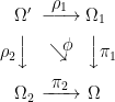
Now consider two separate extensions π1 and π2 of the same underlying probability space,
As maps between sets, these can both be embedded into a single extension known as the pullback or fiber product. This is the set Ω′= Ω1 ×Ω Ω2 defined by
Defining projection maps ρi: Ω′ → Ωi by
results in a commutative square with ϕ ≡ π1○ρ1 = π2○ρ2,
In fact, Ω′ is exactly the cartesian product Ω1 × Ω2 restricted to the subset on which π1○ρ1 and π2○ρ2 agree.
This constructs an extension ϕ of the sample space containing π1 and π2 as sub-extensions. However, it still needs to be made into a probability space. Use the smallest sigma-algebra F ′ on Ω′ making ρ1, ρ2 into measurable maps, which is generated by ρ1∗F 1 ∪ ρ2∗F 2. The probability measure ℙ′ on (Ω′, F ′) is uniquely determined on each of the sub-sigma-algebras by the requirement that ρi preserve probabilities,
for i = 1, 2 and A ∈ F i. These necessarily agree on ϕ∗F ⊆ ρ1∗F 1 ∩ ρ2∗F 2,
for A ∈ F . The natural way to extend ℙ′ to all of F ′ is to use relative independence over ϕ∗F .
Definition 4 The relative product of the extensions π1 and π2 is the extension
with ϕ, Ω′, F ′ constructed as above, and ℙ′ is the unique probability measure for which the projections ρ1, ρ2 preserve probabilities, and for which ρ1∗F 1 and ρ2∗F 2 are relatively independent over ϕ∗F .
A well known fact about joint normally distributed random variables, is that they are independent if and only if their covariance is zero. In one direction, this statement is trivial. Any independent pair of random variables has zero covariance (assuming that they are integrable, so that the covariance has a well-defined value). The strength of the statement is in the other direction. Knowing the value of the covariance does not tell us a lot about the joint distribution so, in the case that they are joint normal, the fact that we can determine independence from this is a rather strong statement.
Theorem 1 A joint normal pair of random variables are independent if and only if their covariance is zero.
Proof: Suppose that X,Y are joint normal, such that and , and that their covariance is c. Then, the characteristic function of can be computed as
for all . It is standard that the joint characteristic function of a pair of random variables is equal to the product of their characteristic functions if and only if they are independent which, in this case, corresponds to the covariance c being zero. ⬜
Example 1 A pair of standard normal random variables X,Y which have zero covariance, but is not normal.
As their sum is not normal, X and Y cannot be independent. This example was constructed by setting for some fixed , which is standard normal whenever X is. As explained in the previous post, the intermediate value theorem ensures that there is a unique value for K making the covariance equal to zero. Continue reading “Independence of Normals”→
I looked at normal random variables in an earlier post but, what does it mean for a sequence of real-valued random variables to be jointly normal? We could simply require each of them to be normal, but this says very little about their joint distribution and is not much help in handling expressions involving more than one of the at once. In case that the random variables are independent, the following result is a very useful property of the normal distribution. All random variables in this post will be real-valued, except where stated otherwise, and we assume that they are defined with respect to some underlying probability space .
Lemma 1 Linear combinations of independent normal random variables are again normal.
Proof: More precisely, if is a sequence of independent normal random variables and are real numbers, then is normal. Let us suppose that has mean and variance . Then, the characteristic function of Y can be computed using the independence property and the characteristic functions of the individual normals,
where we have set and . This is the characteristic function of a normal random variable with mean and variance . ⬜
The definition of joint normal random variables will include the case of independent normals, so that any linear combination is also normal. We use use this result as the defining property for the general multivariate normal case.
Definition 2 A collection of real-valued random variables is multivariate normal (or joint normal) if and only if all of its finite linear combinations are normal.
Figure 1: Probability densities used to extend the zeta function
The famous Riemann zeta function was first introduced by Riemann in order to describe the distribution of the prime numbers. It is defined by the infinite sum
(1)
which is absolutely convergent for all complex s with real part greater than one. One of the first properties of this is that, as shown by Riemann, it extends to an analytic function on the entire complex plane, other than a simple pole at . By the theory of analytic continuation this extension is necessarily unique, so the importance of the result lies in showing that an extension exists. One way of doing this is to find an alternative expression for the zeta function which is well defined everywhere. For example, it can be expressed as an absolutely convergent integral, as performed by Riemann himself in his original 1859 paper on the subject. This leads to an explicit expression for the zeta function, scaled by an analytic prefactor, as the integral of multiplied by a function of x over the range . In fact, this can be done in a way such that the function of x is a probability density function, and hence expresses the Riemann zeta function over the entire complex plane in terms of the generating function of a positive random variable X. The probability distributions involved here are not the standard ones taught to students of probability theory, so may be new to many people. Although these distributions are intimately related to the Riemann zeta function they also, intriguingly, turn up in seemingly unrelated contexts involving Brownian motion.
The normal (or Gaussian) distribution is ubiquitous throughout probability theory for various reasons, including the central limit theorem, the fact that it is realistic for many practical applications, and because it satisfies nice properties making it amenable to mathematical manipulation. It is, therefore, one of the first continuous distributions that students encounter at school. As such, it is not something that I have spent much time discussing on this blog, which is usually concerned with more advanced topics. However, there are many nice properties and methods that can be performed with normal distributions, greatly simplifying the manipulation of expressions in which it is involved. While it is usually possible to ignore these, and instead just substitute in the density function and manipulate the resulting integrals, that approach can get very messy. So, I will describe some of the basic results and ideas that I use frequently.
Throughout, I assume the existence of an underlying probability space . Recall that a real-valued random variable X has the standard normal distribution if it has a probability density function given by,
For it to function as a probability density, it is necessary that it integrates to one. While it is not obvious that the normalization factor is the correct value for this to be true, it is the one fact that I state here without proof. Wikipedia does list a couple of proofs, which can be referred to. By symmetry, and have the same distribution, so that they have the same mean and, therefore, .
The derivative of the density function satisfies the useful identity
(1)
This allows us to quickly verify that standard normal variables have unit variance, by an application of integration by parts.
Another identity satisfied by the normal density function is,
(2)
This enables us to prove the following very useful result. In fact, it is difficult to overstate how helpful this result can be. I make use of it frequently when manipulating expressions involving normal variables, as it significantly simplifies the calculations. It is also easy to remember, and simple to derive if needed.
Theorem 1 Let X be standard normal and be measurable. Then, for all ,
Let me ask the following very simple question. Suppose that I toss a pair of identical coins at the same time, then what is the probability of them both coming up heads? There is no catch here, both coins are fair. There are three possible outcomes, both tails, one head and one tail, and both heads. Assuming that it is completely random so that all outcomes are equally likely, then we could argue that each possibility has a one in three chance of occurring, so that the answer to the question is that the probability is 1/3.
Of course, this is wrong! A fair coin has a probability of 1/2 of showing heads and, by independence, standard probability theory says that we should multiply these together for each coin to get the correct answer of , which can be verified by experiment. Alternatively, we can note that the outcome of one tail and one head, in reality, consists of two equally likely possibilities. Either the first coin can be a head and the second a tail, or vice-versa. So, there are actually four equally likely possible outcomes, only one of which has both coins showing heads, again giving a probability of 1/4. Continue reading “Quantum Coin Tossing”→


![\displaystyle \begin{aligned} \phi_n(\alpha,\beta)&={\mathbb E}\left[e^{i\alpha R_n+i\beta(R_n-S_n)}\right],\\ w_n(\alpha,\beta)&={\mathbb E}\left[e^{i\alpha S_n^++i\beta S_n^-}\right]\\ &={\mathbb E}\left[e^{i\alpha S_n^+}\right]+{\mathbb E}\left[e^{i\beta S_n^-}\right]-1. \end{aligned}](https://s0.wp.com/latex.php?latex=%5Cdisplaystyle+%5Cbegin%7Baligned%7D+%5Cphi_n%28%5Calpha%2C%5Cbeta%29%26%3D%7B%5Cmathbb+E%7D%5Cleft%5Be%5E%7Bi%5Calpha+R_n%2Bi%5Cbeta%28R_n-S_n%29%7D%5Cright%5D%2C%5C%5C+w_n%28%5Calpha%2C%5Cbeta%29%26%3D%7B%5Cmathbb+E%7D%5Cleft%5Be%5E%7Bi%5Calpha+S_n%5E%2B%2Bi%5Cbeta+S_n%5E-%7D%5Cright%5D%5C%5C+%26%3D%7B%5Cmathbb+E%7D%5Cleft%5Be%5E%7Bi%5Calpha+S_n%5E%2B%7D%5Cright%5D%2B%7B%5Cmathbb+E%7D%5Cleft%5Be%5E%7Bi%5Cbeta+S_n%5E-%7D%5Cright%5D-1.+%5Cend%7Baligned%7D+&bg=ffffff&fg=000000&s=0&c=20201002)

![\displaystyle \begin{aligned} \tilde\phi_n(\alpha,\beta)&={\mathbb E}\left[e^{i\alpha R_n+i\beta S_n}\right],\\ \tilde w_n(\alpha,\beta)&={\mathbb E}\left[e^{i\alpha S_n^++i\beta S_n}\right]. \end{aligned}](https://s0.wp.com/latex.php?latex=%5Cdisplaystyle+%5Cbegin%7Baligned%7D+%5Ctilde%5Cphi_n%28%5Calpha%2C%5Cbeta%29%26%3D%7B%5Cmathbb+E%7D%5Cleft%5Be%5E%7Bi%5Calpha+R_n%2Bi%5Cbeta+S_n%7D%5Cright%5D%2C%5C%5C+%5Ctilde+w_n%28%5Calpha%2C%5Cbeta%29%26%3D%7B%5Cmathbb+E%7D%5Cleft%5Be%5E%7Bi%5Calpha+S_n%5E%2B%2Bi%5Cbeta+S_n%7D%5Cright%5D.+%5Cend%7Baligned%7D+&bg=ffffff&fg=000000&s=0&c=20201002)
![\displaystyle \sum_{n=0}^\infty {\mathbb E}\left[e^{i\alpha R_n}\right]t^n=\exp\left(\sum_{n=1}^\infty {\mathbb E}\left[e^{i\alpha S_n^+}\right]\frac{t^n}n\right)](https://s0.wp.com/latex.php?latex=%5Cdisplaystyle+%5Csum_%7Bn%3D0%7D%5E%5Cinfty+%7B%5Cmathbb+E%7D%5Cleft%5Be%5E%7Bi%5Calpha+R_n%7D%5Cright%5Dt%5En%3D%5Cexp%5Cleft%28%5Csum_%7Bn%3D1%7D%5E%5Cinfty+%7B%5Cmathbb+E%7D%5Cleft%5Be%5E%7Bi%5Calpha+S_n%5E%2B%7D%5Cright%5D%5Cfrac%7Bt%5En%7Dn%5Cright%29+&bg=ffffff&fg=000000&s=0&c=20201002)
![\displaystyle {\mathbb E}[R_n]=\sum_{k=1}^n\frac1k{\mathbb E}[S_k^+].](https://s0.wp.com/latex.php?latex=%5Cdisplaystyle+%7B%5Cmathbb+E%7D%5BR_n%5D%3D%5Csum_%7Bk%3D1%7D%5En%5Cfrac1k%7B%5Cmathbb+E%7D%5BS_k%5E%2B%5D.+&bg=ffffff&fg=000000&s=0&c=20201002)
![\displaystyle \begin{aligned} \sum_{n=0}^\infty i{\mathbb E}[R_n]t^n &=\exp\left(\sum_{n=1}^\infty \frac{t^n}n\right)\sum_{n=1}^\infty i{\mathbb E}[S_n^+]\frac{t^n}n\\ &=\exp\left(-\log(1-t)\right)\sum_{n=1}^\infty i{\mathbb E}[S_n^+]\frac{t^n}n\\ &=(1-t)^{-1}\sum_{n=1}^\infty i{\mathbb E}[S_n^+]\frac{t^n}n\\ &=(1+t+t^2+\cdots)\sum_{n=1}^\infty i{\mathbb E}[S_n^+]\frac{t^n}n. \end{aligned}](https://s0.wp.com/latex.php?latex=%5Cdisplaystyle+%5Cbegin%7Baligned%7D+%5Csum_%7Bn%3D0%7D%5E%5Cinfty+i%7B%5Cmathbb+E%7D%5BR_n%5Dt%5En+%26%3D%5Cexp%5Cleft%28%5Csum_%7Bn%3D1%7D%5E%5Cinfty+%5Cfrac%7Bt%5En%7Dn%5Cright%29%5Csum_%7Bn%3D1%7D%5E%5Cinfty+i%7B%5Cmathbb+E%7D%5BS_n%5E%2B%5D%5Cfrac%7Bt%5En%7Dn%5C%5C+%26%3D%5Cexp%5Cleft%28-%5Clog%281-t%29%5Cright%29%5Csum_%7Bn%3D1%7D%5E%5Cinfty+i%7B%5Cmathbb+E%7D%5BS_n%5E%2B%5D%5Cfrac%7Bt%5En%7Dn%5C%5C+%26%3D%281-t%29%5E%7B-1%7D%5Csum_%7Bn%3D1%7D%5E%5Cinfty+i%7B%5Cmathbb+E%7D%5BS_n%5E%2B%5D%5Cfrac%7Bt%5En%7Dn%5C%5C+%26%3D%281%2Bt%2Bt%5E2%2B%5Ccdots%29%5Csum_%7Bn%3D1%7D%5E%5Cinfty+i%7B%5Cmathbb+E%7D%5BS_n%5E%2B%5D%5Cfrac%7Bt%5En%7Dn.+%5Cend%7Baligned%7D+&bg=ffffff&fg=000000&s=0&c=20201002)


![\displaystyle {\mathbb P}(\lvert Z\rvert > x)\ge\frac{({\mathbb E}\lvert Z\rvert-x)^2}{{\mathbb E}[Z^2]}](https://s0.wp.com/latex.php?latex=%5Cdisplaystyle+%7B%5Cmathbb+P%7D%28%5Clvert+Z%5Crvert+%3E+x%29%5Cge%5Cfrac%7B%28%7B%5Cmathbb+E%7D%5Clvert+Z%5Crvert-x%29%5E2%7D%7B%7B%5Cmathbb+E%7D%5BZ%5E2%5D%7D+&bg=ffffff&fg=000000&s=0&c=20201002)

![\displaystyle {\mathbb E}[Z^2]=\lVert a\rVert_2^2=\sum_na_n^2.](https://s0.wp.com/latex.php?latex=%5Cdisplaystyle+%7B%5Cmathbb+E%7D%5BZ%5E2%5D%3D%5ClVert+a%5CrVert_2%5E2%3D%5Csum_na_n%5E2.+&bg=ffffff&fg=000000&s=0&c=20201002)


 , which I will also shorten to
  . An explicit construction of a non-Borel set was given by Lusin in 1927. Every irrational real number can be expressed uniquely as a

 consisting of sigma-algebra
  on set
  consists of all subsets
  with
with  is the Lebesgue sigma-algebra, which I will denote by
  . Usually, when saying that a subset of the reals is measurable without further qualification, it is understood to mean that it is in
  consists of the subsets of
 .
. consisting of all subsets of a set
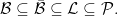


![\displaystyle {\mathbb P}(A\cap B) = {\mathbb E}\left[{\mathbb P}(A\vert\mathcal K){\mathbb P}(B\vert\mathcal K)\right]](https://s0.wp.com/latex.php?latex=%5Cdisplaystyle+%7B%5Cmathbb+P%7D%28A%5Ccap+B%29+%3D+%7B%5Cmathbb+E%7D%5Cleft%5B%7B%5Cmathbb+P%7D%28A%5Cvert%5Cmathcal+K%29%7B%5Cmathbb+P%7D%28B%5Cvert%5Cmathcal+K%29%5Cright%5D+&bg=ffffff&fg=000000&s=0&c=20201002)


 and
and  , and that their covariance is c. Then, the characteristic function of
![\displaystyle \begin{aligned} {\mathbb E}\left[e^{iaX+ibY}\right] &=e^{ia\mu_X+ib\mu_Y-\frac12(a^2\sigma_X^2+2abc+b^2\sigma_Y^2)}\\ &=e^{-abc}{\mathbb E}\left[e^{iaX}\right]{\mathbb E}\left[e^{ibY}\right] \end{aligned}](https://s0.wp.com/latex.php?latex=%5Cdisplaystyle++%5Cbegin%7Baligned%7D+%7B%5Cmathbb+E%7D%5Cleft%5Be%5E%7BiaX%2BibY%7D%5Cright%5D+%26%3De%5E%7Bia%5Cmu_X%2Bib%5Cmu_Y-%5Cfrac12%28a%5E2%5Csigma_X%5E2%2B2abc%2Bb%5E2%5Csigma_Y%5E2%29%7D%5C%5C+%26%3De%5E%7B-abc%7D%7B%5Cmathbb+E%7D%5Cleft%5Be%5E%7BiaX%7D%5Cright%5D%7B%5Cmathbb+E%7D%5Cleft%5Be%5E%7BibY%7D%5Cright%5D+%5Cend%7Baligned%7D+&bg=ffffff&fg=000000&s=0&c=20201002)
 . It is standard that the joint characteristic function of a pair of random variables is equal to the product of their characteristic functions if and only if they are independent which, in this case, corresponds to the covariance c being zero. ⬜
 is not normal.
  for some fixed
  , which is standard normal whenever X is. As explained in the previous post, the intermediate value theorem ensures that there is a unique value for K making the covariance
 ![{{\mathbb E}[XY]}](https://s0.wp.com/latex.php?latex=%7B%7B%5Cmathbb+E%7D%5BXY%5D%7D&bg=ffffff&fg=000000&s=0&c=20201002) equal to zero.
equal to zero.  to be jointly normal? We could simply require each of them to be normal, but this says very little about their joint distribution and is not much help in handling expressions involving more than one of the
  at once. In case that the random variables are independent, the following result is a very useful property of the normal distribution. All random variables in this post will be real-valued, except where stated otherwise, and we assume that they are defined with respect to some underlying probability space
  .
. is a sequence of independent normal random variables and
  are real numbers, then
  is normal. Let us suppose that
  has mean
  and variance
  . Then, the characteristic function of Y can be computed using the independence property and the
 ![\displaystyle \begin{aligned} {\mathbb E}\left[e^{i\lambda Y}\right] &={\mathbb E}\left[\prod_ke^{i\lambda a_k X_k}\right] =\prod_k{\mathbb E}\left[e^{i\lambda a_k X_k}\right]\\ &=\prod_ke^{-\frac12\lambda^2a_k^2\sigma_k^2+i\lambda a_k\mu_k} =e^{-\frac12\lambda^2\sigma^2+i\lambda\mu} \end{aligned}](https://s0.wp.com/latex.php?latex=%5Cdisplaystyle++%5Cbegin%7Baligned%7D+%7B%5Cmathbb+E%7D%5Cleft%5Be%5E%7Bi%5Clambda+Y%7D%5Cright%5D+%26%3D%7B%5Cmathbb+E%7D%5Cleft%5B%5Cprod_ke%5E%7Bi%5Clambda+a_k+X_k%7D%5Cright%5D+%3D%5Cprod_k%7B%5Cmathbb+E%7D%5Cleft%5Be%5E%7Bi%5Clambda+a_k+X_k%7D%5Cright%5D%5C%5C+%26%3D%5Cprod_ke%5E%7B-%5Cfrac12%5Clambda%5E2a_k%5E2%5Csigma_k%5E2%2Bi%5Clambda+a_k%5Cmu_k%7D+%3De%5E%7B-%5Cfrac12%5Clambda%5E2%5Csigma%5E2%2Bi%5Clambda%5Cmu%7D+%5Cend%7Baligned%7D+&bg=ffffff&fg=000000&s=0&c=20201002)
 and
and  . This is the characteristic function of a normal random variable with mean
  and variance
  . ⬜
. ⬜ of real-valued random variables is multivariate normal (or joint normal) if and only if all of its finite linear combinations are normal.

 . By the theory of
  multiplied by a function of x over the range
  . In fact, this can be done in a way such that the function of x is a probability density function, and hence expresses the Riemann zeta function over the entire complex plane in terms of the generating function
 ![{{\mathbb E}[X^s]}](https://s0.wp.com/latex.php?latex=%7B%7B%5Cmathbb+E%7D%5BX%5Es%5D%7D&bg=ffffff&fg=000000&s=0&c=20201002) of a positive random variable X. The probability distributions involved here are not the standard ones taught to students of probability theory, so may be new to many people. Although these distributions are intimately related to the Riemann zeta function they also, intriguingly, turn up in seemingly unrelated contexts involving Brownian motion.
of a positive random variable X. The probability distributions involved here are not the standard ones taught to students of probability theory, so may be new to many people. Although these distributions are intimately related to the Riemann zeta function they also, intriguingly, turn up in seemingly unrelated contexts involving Brownian motion.
 is the correct value for this to be true, it is the one fact that I state here without proof.
  and
and  have the same distribution, so that they have the same mean and, therefore,
 ![{{\mathbb E}[X]=0}](https://s0.wp.com/latex.php?latex=%7B%7B%5Cmathbb+E%7D%5BX%5D%3D0%7D&bg=ffffff&fg=000000&s=0&c=20201002) .
.
![\displaystyle \begin{aligned} {\mathbb E}[X^2] &=\int x^2\varphi(x)dx\\ &= -\int x\varphi^\prime(x)dx\\ &=\int\varphi(x)dx-[x\varphi(x)]_{-\infty}^\infty=1 \end{aligned}](https://s0.wp.com/latex.php?latex=%5Cdisplaystyle++%5Cbegin%7Baligned%7D+%7B%5Cmathbb+E%7D%5BX%5E2%5D+%26%3D%5Cint+x%5E2%5Cvarphi%28x%29dx%5C%5C+%26%3D+-%5Cint+x%5Cvarphi%5E%5Cprime%28x%29dx%5C%5C+%26%3D%5Cint%5Cvarphi%28x%29dx-%5Bx%5Cvarphi%28x%29%5D_%7B-%5Cinfty%7D%5E%5Cinfty%3D1+%5Cend%7Baligned%7D+&bg=ffffff&fg=000000&s=0&c=20201002)

 be measurable. Then, for all
  ,
, ![\displaystyle \begin{aligned} {\mathbb E}[e^{\lambda X}f(X)] &={\mathbb E}[e^{\lambda X}]{\mathbb E}[f(X+\lambda)]\\ &=e^{\frac{\lambda^2}{2}}{\mathbb E}[f(X+\lambda)]. \end{aligned}](https://s0.wp.com/latex.php?latex=%5Cdisplaystyle++%5Cbegin%7Baligned%7D+%7B%5Cmathbb+E%7D%5Be%5E%7B%5Clambda+X%7Df%28X%29%5D+%26%3D%7B%5Cmathbb+E%7D%5Be%5E%7B%5Clambda+X%7D%5D%7B%5Cmathbb+E%7D%5Bf%28X%2B%5Clambda%29%5D%5C%5C+%26%3De%5E%7B%5Cfrac%7B%5Clambda%5E2%7D%7B2%7D%7D%7B%5Cmathbb+E%7D%5Bf%28X%2B%5Clambda%29%5D.+%5Cend%7Baligned%7D+&bg=ffffff&fg=000000&s=0&c=20201002)

 , which can be verified by experiment. Alternatively, we can note that the outcome of one tail and one head, in reality, consists of two equally likely possibilities. Either the first coin can be a head and the second a tail, or vice-versa. So, there are actually four equally likely possible outcomes, only one of which has both coins showing heads, again giving a probability of 1/4.