

The famous Riemann zeta function was first introduced by Riemann in order to describe the distribution of the prime numbers. It is defined by the infinite sum
 |
(1) |
which is absolutely convergent for all complex s with real part greater than one. One of the first properties of this is that, as shown by Riemann, it extends to an analytic function on the entire complex plane, other than a simple pole at 


![{{\mathbb E}[X^s]}](https://s0.wp.com/latex.php?latex=%7B%7B%5Cmathbb+E%7D%5BX%5Es%5D%7D&bg=ffffff&fg=000000&s=0&c=20201002)
In this post, I derive two probability distributions related to the extension of the Riemann zeta function, and describe some of their properties. I also show how they can be constructed as the sum of a sequence of gamma distributed random variables. For motivation, some examples are given of where they show up in apparently unrelated areas of probability theory, although I do not give proofs of these statements here. For more information, see the 2001 paper Probability laws related to the Jacobi theta and Riemann zeta functions, and Brownian excursions by Biane, Pitman, and Yor.
The functional equation discovered by Riemann relates the values of 


 |
Here, 
 |
over 

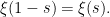 |
It can be shown that 


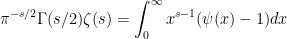
I will now outline a method of extending the zeta and xi functions and of deriving the functional equation, showing how it involves a probability distribution. We start with a simple rearrangement of a particular integral. Fixing a positive constant 

 |
(2) |
Hence, the definition of the zeta function over
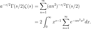 |
Before taking this further, I mention the Jacobi identity, which applies to the summation inside the integral above. This is,
 |
for all real 


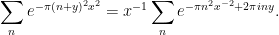 |
(3) |
Note that the left hand side is periodic in y with period 1, and its Fourier series expansion can be computed, giving the right hand side. In particular, setting 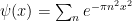

 |
Now, multiply through by 


 |
The third equality is just integration by parts, so we have obtained
 |
(4) |
where 
 |
(5) |
We note that this vanishes quickly as x goes to infinity.
Lemma 1 The following asymptotic limit holds as x tends to infinity,
(6)
Proof: Definition (5) gives
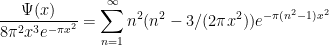 |
and, by dominated convergence, we can take the limit 

In particular, 
 |
(7) |
So, 


 |
Looking at the function
Theorem 2 The function
(8) for all
.
![\displaystyle {\mathbb E}[X^s]=2\xi(s)](https://s0.wp.com/latex.php?latex=%5Cdisplaystyle++%7B%5Cmathbb+E%7D%5BX%5Es%5D%3D2%5Cxi%28s%29+&bg=ffffff&fg=000000&s=0&c=20201002)
Proof: For all 
 |
and, hence, (5) gives 

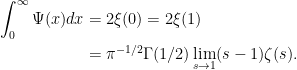 |
The identity 


Equation (8) describes the moments of a random variable X with probability density 

![\displaystyle \begin{aligned} &{\mathbb E}[X]=1,\\ &{\mathbb E}[X^2]=\frac\pi3. \end{aligned}](https://s0.wp.com/latex.php?latex=%5Cdisplaystyle++%5Cbegin%7Baligned%7D+%26%7B%5Cmathbb+E%7D%5BX%5D%3D1%2C%5C%5C+%26%7B%5Cmathbb+E%7D%5BX%5E2%5D%3D%5Cfrac%5Cpi3.+%5Cend%7Baligned%7D+&bg=ffffff&fg=000000&s=0&c=20201002) |
As an example of an apparently unrelated situation where this distribution occurs, consider a standard Brownian bridge ![{\{B_t\}_{t\in[0,1]}}](https://s0.wp.com/latex.php?latex=%7B%5C%7BB_t%5C%7D_%7Bt%5Cin%5B0%2C1%5D%7D%7D&bg=ffffff&fg=000000&s=0&c=20201002)

 |
Up to a constant scaling factor, this has probability density 


![\displaystyle \begin{aligned} &Z=\max_{0\le s\le t\le1}\lvert B_t-B_s+(s-t)B_1\rvert\\ &{\mathbb E}\left[Z^u\right]=2^{-\frac u2}u(u-1)\Gamma\left(\frac u2\right)\zeta(u). \end{aligned}](https://s0.wp.com/latex.php?latex=%5Cdisplaystyle++%5Cbegin%7Baligned%7D+%26Z%3D%5Cmax_%7B0%5Cle+s%5Cle+t%5Cle1%7D%5Clvert+B_t-B_s%2B%28s-t%29B_1%5Crvert%5C%5C+%26%7B%5Cmathbb+E%7D%5Cleft%5BZ%5Eu%5Cright%5D%3D2%5E%7B-%5Cfrac+u2%7Du%28u-1%29%5CGamma%5Cleft%28%5Cfrac+u2%5Cright%29%5Czeta%28u%29.+%5Cend%7Baligned%7D+&bg=ffffff&fg=000000&s=0&c=20201002) |
At the time of writing, these are the equations on the notepad in the banner image of this site.
Another example is given by normalised Brownian excursions, which can be constructed as a Brownian bridge conditioned on being nonnegative. The maximum value of the excursion, again after scaling by
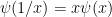
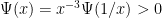
Riemann’s functional equation can alternatively be expressed as a symmetry of of the probability distribution introduced above.
Theorem 3 (The Functional Equation) Let X be a positive random variable with probability density
(9) for all measurable functions
.
![\displaystyle {\mathbb E}[Xf(1/X)]={\mathbb E}[f(X)]](https://s0.wp.com/latex.php?latex=%5Cdisplaystyle++%7B%5Cmathbb+E%7D%5BXf%281%2FX%29%5D%3D%7B%5Cmathbb+E%7D%5Bf%28X%29%5D+&bg=ffffff&fg=000000&s=0&c=20201002)
Proof: We can define a new measure 
![\displaystyle {\mathbb E}_{\mathbb Q}[f(X)]={\mathbb E}[Xf(1/X)]](https://s0.wp.com/latex.php?latex=%5Cdisplaystyle++%7B%5Cmathbb+E%7D_%7B%5Cmathbb+Q%7D%5Bf%28X%29%5D%3D%7B%5Cmathbb+E%7D%5BXf%281%2FX%29%5D+&bg=ffffff&fg=000000&s=0&c=20201002) |
for all measurable functions
![\displaystyle {\mathbb E}_{\mathbb Q}[X^{s}]={\mathbb E}[X/X^{s}]=2\xi(1-s)=2\xi(s)={\mathbb E}[X^{s}]](https://s0.wp.com/latex.php?latex=%5Cdisplaystyle++%7B%5Cmathbb+E%7D_%7B%5Cmathbb+Q%7D%5BX%5E%7Bs%7D%5D%3D%7B%5Cmathbb+E%7D%5BX%2FX%5E%7Bs%7D%5D%3D2%5Cxi%281-s%29%3D2%5Cxi%28s%29%3D%7B%5Cmathbb+E%7D%5BX%5E%7Bs%7D%5D+&bg=ffffff&fg=000000&s=0&c=20201002) |
for real s. Taking 
![{{\mathbb E}_{\mathbb Q}[1]=1}](https://s0.wp.com/latex.php?latex=%7B%7B%5Cmathbb+E%7D_%7B%5Cmathbb+Q%7D%5B1%5D%3D1%7D&bg=ffffff&fg=000000&s=0&c=20201002)

Actually, identity (9) is equivalent to the functional equation. By linearity, it extends to any 


![\displaystyle 2\xi(1-s)={\mathbb E}[X^{1-s}]={\mathbb E}[X/X^s]={\mathbb E}[X^s]=2\xi(s).](https://s0.wp.com/latex.php?latex=%5Cdisplaystyle++2%5Cxi%281-s%29%3D%7B%5Cmathbb+E%7D%5BX%5E%7B1-s%7D%5D%3D%7B%5Cmathbb+E%7D%5BX%2FX%5Es%5D%3D%7B%5Cmathbb+E%7D%5BX%5Es%5D%3D2%5Cxi%28s%29.+&bg=ffffff&fg=000000&s=0&c=20201002) |
Interestingly, we have seen the symmetry (9) previously in these notes for an entirely different distribution. Lemma 10 of the post on the normal distribution states that it holds for any lognormal random variable X of mean 1.
Another Distribution
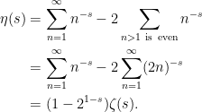
Instead of starting with the usual series (1) defining the Riemann zeta function, we can instead consider a similar series which has alternating signs, giving the Dirichlet eta function
 |
This has the benefit of converging for all
 |
In a similar fashion to the derivation above, we apply identity (2) with 
 |
where we set
 |
(10) |
Applying integration by parts, we have obtained
 |
(11) |
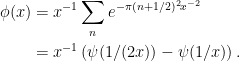
where I define
 |
A Jacobi style identity is also satisfied by 


 |
(12) |
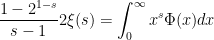
Hence, 
 |
(13) |
These expressions show that 


 |
This is a differential equation for
 |
(14) |
This leads us to another probability density.
Theorem 4 The function
(15) for all
![\displaystyle \begin{aligned} E[X^s] &=s(1-2^{1-s})\pi^{-s/2}\Gamma(s/2)\zeta(s)\\ &= \frac{1-2^{1-s}}{s-1}2\xi(s) \end{aligned}](https://s0.wp.com/latex.php?latex=%5Cdisplaystyle++%5Cbegin%7Baligned%7D+E%5BX%5Es%5D+%26%3Ds%281-2%5E%7B1-s%7D%29%5Cpi%5E%7B-s%2F2%7D%5CGamma%28s%2F2%29%5Czeta%28s%29%5C%5C+%26%3D+%5Cfrac%7B1-2%5E%7B1-s%7D%7D%7Bs-1%7D2%5Cxi%28s%29+%5Cend%7Baligned%7D+&bg=ffffff&fg=000000&s=0&c=20201002)
Proof: Equation (14) together with positivity of
 |
as required. Finally, (15) follows from (11). ⬜
As an example of where this second probability distribution appears in a context apparently unrelated to the Riemann zeta function, consider an IID sequence of random variables 

 |
The maximum discrepancy between this sample distribution function and the true underlying one is,
 |
This is a random quantity which, after scaling by the factor 

Another example is given by a standard Brownian bridge B. The scaled absolute maximum 
 |
after scaling by a factor 
A further example is provided by a Brownian meander ![{[0,1]}](https://s0.wp.com/latex.php?latex=%7B%5B0%2C1%5D%7D&bg=ffffff&fg=000000&s=0&c=20201002)

Properties of the Distributions
I will now describe and prove some of the properties of the distributions, including computing their cumulative distribution and moment generating functions. I also show how they can be realized as a sum of gamma distributed random variables. First, the two probability densities are related in the following simple but surprising way.
Lemma 5 Let X have probability density
. Then,
has probability density
Proof: The generating function of 
![\displaystyle \begin{aligned} {\mathbb E}[Z^s] &={\mathbb E}[Y^{-s}]{\mathbb E}[X^s]\\ &=\int_1^2y^{-s}dy\,2\xi(s)\\ &=\frac{1-2^{1-s}}{s-1}2\xi(s) \end{aligned}](https://s0.wp.com/latex.php?latex=%5Cdisplaystyle++%5Cbegin%7Baligned%7D+%7B%5Cmathbb+E%7D%5BZ%5Es%5D+%26%3D%7B%5Cmathbb+E%7D%5BY%5E%7B-s%7D%5D%7B%5Cmathbb+E%7D%5BX%5Es%5D%5C%5C+%26%3D%5Cint_1%5E2y%5E%7B-s%7Ddy%5C%2C2%5Cxi%28s%29%5C%5C+%26%3D%5Cfrac%7B1-2%5E%7B1-s%7D%7D%7Bs-1%7D2%5Cxi%28s%29+%5Cend%7Baligned%7D+&bg=ffffff&fg=000000&s=0&c=20201002) |
which, according to (15), is the generating function corresponding to a variable with probability density
Less surprisingly, the cumulative distribution functions can be computed directly from the definitions above.
Lemma 6 If X has probability density
(16) If it has probability density
(17)


Proof: For the first equation, if X has probability density 
 |
For equation (17), equality of each of the three expressions on the right hand side is given by differentiating the defining series of 

 |
⬜
The calculation of the moment generating functions will require the following integral identity due to Lévy.
Lemma 7 For any positive reals
, the integral identity
(18) holds.
Proof: Using the substitution 
 |
The integral in the lemma can be split into the ranges 

 |
Next, apply the substitution 
 |
which transforms the integral to,
 |
as required. ⬜
We now compute the moment generating functions for squares of random variables with the distributions above. The results are surprisingly simple, and it is not clear why this should be so.
Lemma 8 If X has probability density
for all real
. If X has probability density
![\displaystyle {\mathbb E}\left[e^{-\pi^{-1}\lambda^2X^2}\right]=\frac{\lambda}{\sinh\lambda}](https://s0.wp.com/latex.php?latex=%5Cdisplaystyle++%7B%5Cmathbb+E%7D%5Cleft%5Be%5E%7B-%5Cpi%5E%7B-1%7D%5Clambda%5E2X%5E2%7D%5Cright%5D%3D%5Cfrac%7B%5Clambda%7D%7B%5Csinh%5Clambda%7D+&bg=ffffff&fg=000000&s=0&c=20201002)
![\displaystyle {\mathbb E}\left[e^{-\pi^{-1}\lambda^2X^2}\right]=\left(\frac{\lambda}{\sinh\lambda}\right)^2.](https://s0.wp.com/latex.php?latex=%5Cdisplaystyle++%7B%5Cmathbb+E%7D%5Cleft%5Be%5E%7B-%5Cpi%5E%7B-1%7D%5Clambda%5E2X%5E2%7D%5Cright%5D%3D%5Cleft%28%5Cfrac%7B%5Clambda%7D%7B%5Csinh%5Clambda%7D%5Cright%29%5E2.+&bg=ffffff&fg=000000&s=0&c=20201002)
Proof: As the exponential term inside the expectations tends to 1 as X goes to zero, rather than vanishing, we use the form for the probability densities which explicitly vanish at zero, to ensure integrability of all the terms. If X has probability density 
![\displaystyle \begin{aligned} {\mathbb E}\left[e^{\pi^{-1}\lambda^2X^2}\right] &=\int_0^\infty \phi^\prime(x)e^{-\pi^{-1}\lambda^2 x^2}dx\\ &=2\lambda\int_0^\infty \pi^{-1}\lambda x\phi(x)e^{-\pi^{-1}\lambda^2 x^2}dx\\ &=4\lambda\sum_{n=0}^\infty\int_0^\infty\pi^{-1}\lambda e^{-\pi^{-1}\lambda^2 x^2-\pi(n+1/2)^2x^{-2}}dx\\ &=2\lambda\sum_{n=0}^\infty e^{-\lambda(2n+1)} =2\lambda e^{-\lambda}/(1-e^{-2\lambda})\\ &=\lambda/\sinh\lambda \end{aligned}](https://s0.wp.com/latex.php?latex=%5Cdisplaystyle++%5Cbegin%7Baligned%7D+%7B%5Cmathbb+E%7D%5Cleft%5Be%5E%7B%5Cpi%5E%7B-1%7D%5Clambda%5E2X%5E2%7D%5Cright%5D+%26%3D%5Cint_0%5E%5Cinfty+%5Cphi%5E%5Cprime%28x%29e%5E%7B-%5Cpi%5E%7B-1%7D%5Clambda%5E2+x%5E2%7Ddx%5C%5C+%26%3D2%5Clambda%5Cint_0%5E%5Cinfty+%5Cpi%5E%7B-1%7D%5Clambda+x%5Cphi%28x%29e%5E%7B-%5Cpi%5E%7B-1%7D%5Clambda%5E2+x%5E2%7Ddx%5C%5C+%26%3D4%5Clambda%5Csum_%7Bn%3D0%7D%5E%5Cinfty%5Cint_0%5E%5Cinfty%5Cpi%5E%7B-1%7D%5Clambda+e%5E%7B-%5Cpi%5E%7B-1%7D%5Clambda%5E2+x%5E2-%5Cpi%28n%2B1%2F2%29%5E2x%5E%7B-2%7D%7Ddx%5C%5C+%26%3D2%5Clambda%5Csum_%7Bn%3D0%7D%5E%5Cinfty+e%5E%7B-%5Clambda%282n%2B1%29%7D+%3D2%5Clambda+e%5E%7B-%5Clambda%7D%2F%281-e%5E%7B-2%5Clambda%7D%29%5C%5C+%26%3D%5Clambda%2F%5Csinh%5Clambda+%5Cend%7Baligned%7D+&bg=ffffff&fg=000000&s=0&c=20201002) |
as required. Here, (18) was used to perform the integral.
Next, suppose that X has probability density 
 |
Using integration by parts, and the notation 

![\displaystyle \begin{aligned} {\mathbb E}\left[e^{\pi^{-1}\lambda^2X^2}\right] &=\int_0^\infty (x\psi(x))^{\prime\prime}e^{-\pi^{-1}\lambda^2 x^2}dx\\ &=\int_0^\infty(4\pi^{-2}\lambda^4x^2-2\pi^{-1}\lambda^2) (x\psi(x)-1) e^{-\pi^{-1}\lambda^2 x^2}dx\\ &=-2\lambda^2\partial_\lambda\int_0^\infty\pi^{-1}\lambda (x\psi(x)-1) e^{-\pi^{-1}\lambda^2 x^2}dx\\ &=-4\lambda^2\partial_\lambda\sum_{n=1}^\infty\int_0^\infty\pi^{-1}\lambda e^{-\pi^{-1}\lambda^2 x^2-\pi n^2 x^{-2}}dx\\ &=-2\lambda^2\partial_\lambda\sum_{n=1}^\infty e^{-2\lambda n} =-2\lambda^2\partial_\lambda(1/(e^{2\lambda}-1))\\ &=4\lambda^2e^{2\lambda}/(e^{2\lambda}-1)^2 =(\lambda/\sinh\lambda)^2 \end{aligned}](https://s0.wp.com/latex.php?latex=%5Cdisplaystyle++%5Cbegin%7Baligned%7D+%7B%5Cmathbb+E%7D%5Cleft%5Be%5E%7B%5Cpi%5E%7B-1%7D%5Clambda%5E2X%5E2%7D%5Cright%5D+%26%3D%5Cint_0%5E%5Cinfty+%28x%5Cpsi%28x%29%29%5E%7B%5Cprime%5Cprime%7De%5E%7B-%5Cpi%5E%7B-1%7D%5Clambda%5E2+x%5E2%7Ddx%5C%5C+%26%3D%5Cint_0%5E%5Cinfty%284%5Cpi%5E%7B-2%7D%5Clambda%5E4x%5E2-2%5Cpi%5E%7B-1%7D%5Clambda%5E2%29+%28x%5Cpsi%28x%29-1%29+e%5E%7B-%5Cpi%5E%7B-1%7D%5Clambda%5E2+x%5E2%7Ddx%5C%5C+%26%3D-2%5Clambda%5E2%5Cpartial_%5Clambda%5Cint_0%5E%5Cinfty%5Cpi%5E%7B-1%7D%5Clambda+%28x%5Cpsi%28x%29-1%29+e%5E%7B-%5Cpi%5E%7B-1%7D%5Clambda%5E2+x%5E2%7Ddx%5C%5C+%26%3D-4%5Clambda%5E2%5Cpartial_%5Clambda%5Csum_%7Bn%3D1%7D%5E%5Cinfty%5Cint_0%5E%5Cinfty%5Cpi%5E%7B-1%7D%5Clambda+e%5E%7B-%5Cpi%5E%7B-1%7D%5Clambda%5E2+x%5E2-%5Cpi+n%5E2+x%5E%7B-2%7D%7Ddx%5C%5C+%26%3D-2%5Clambda%5E2%5Cpartial_%5Clambda%5Csum_%7Bn%3D1%7D%5E%5Cinfty+e%5E%7B-2%5Clambda+n%7D+%3D-2%5Clambda%5E2%5Cpartial_%5Clambda%281%2F%28e%5E%7B2%5Clambda%7D-1%29%29%5C%5C+%26%3D4%5Clambda%5E2e%5E%7B2%5Clambda%7D%2F%28e%5E%7B2%5Clambda%7D-1%29%5E2+%3D%28%5Clambda%2F%5Csinh%5Clambda%29%5E2+%5Cend%7Baligned%7D+&bg=ffffff&fg=000000&s=0&c=20201002) |
as required. ⬜
Knowing the moment generating functions opens up a world of possibilities. For example, we find the following simple relation between the two distributions.
Lemma 9 Let X and Y be independent random variables with probability density
has probability density
Proof: The moment generating function of 
![\displaystyle \begin{aligned} {\mathbb E}[e^{-\pi^{-1}\lambda^2Z^2}] &= {\mathbb E}[e^{-\pi^{-1}\lambda^2X^2}] {\mathbb E}[e^{-\pi^{-1}\lambda^2Y^2}]\\ &=(\lambda/\sinh\lambda)^2. \end{aligned}](https://s0.wp.com/latex.php?latex=%5Cdisplaystyle++%5Cbegin%7Baligned%7D+%7B%5Cmathbb+E%7D%5Be%5E%7B-%5Cpi%5E%7B-1%7D%5Clambda%5E2Z%5E2%7D%5D+%26%3D+%7B%5Cmathbb+E%7D%5Be%5E%7B-%5Cpi%5E%7B-1%7D%5Clambda%5E2X%5E2%7D%5D+%7B%5Cmathbb+E%7D%5Be%5E%7B-%5Cpi%5E%7B-1%7D%5Clambda%5E2Y%5E2%7D%5D%5C%5C+%26%3D%28%5Clambda%2F%5Csinh%5Clambda%29%5E2.+%5Cend%7Baligned%7D+&bg=ffffff&fg=000000&s=0&c=20201002) |
Applying lemma 8 again and using the fact that the distribution of a nonnegative random variable is uniquely determined by its moment generating function shows that Z has probability density
We now have lemma 5 which give us a method of converting a random variable with density
Corollary 10 Let X,Y,U,V be independent random variables with U,V uniform on
- If X,Y have probability density
.
- If X,Y have probability density
.
Proof: For the first statement,
For the second statement, 

In fact, it is not difficult to show that the properties given by corollary 10 uniquely determine the probability distributions, up to a constant scaling factor. This can be done by iteratively applying the statements to approximate the distributions in terms of a sum over products of inverse squares of uniform random variables. I do not go through this here though, and instead show how we can construct random variables with the given densities as a sum of gamma distributed random variables.
Recall that, for real 


Theorem 11 Let
be an IID sequence of nonnegative random variables with the
This has moment generating function
(19) for real
- if
then
has probability density
- if
then

![\displaystyle {\mathbb E}[e^{-\lambda^2 X}]=\left(\frac{\lambda}{\sinh\lambda}\right)^a](https://s0.wp.com/latex.php?latex=%5Cdisplaystyle++%7B%5Cmathbb+E%7D%5Be%5E%7B-%5Clambda%5E2+X%7D%5D%3D%5Cleft%28%5Cfrac%7B%5Clambda%7D%7B%5Csinh%5Clambda%7D%5Cright%29%5Ea+&bg=ffffff&fg=000000&s=0&c=20201002)
Proof: As it has the gamma distribution with parameter 
![\displaystyle {\mathbb E}[e^{-u Z_n}]=\Gamma(a)^{-1}\int_0^\infty z^{a-1}e^{-(1+u)z}dz=(1+u)^{-a}.](https://s0.wp.com/latex.php?latex=%5Cdisplaystyle++%7B%5Cmathbb+E%7D%5Be%5E%7B-u+Z_n%7D%5D%3D%5CGamma%28a%29%5E%7B-1%7D%5Cint_0%5E%5Cinfty+z%5E%7Ba-1%7De%5E%7B-%281%2Bu%29z%7Ddz%3D%281%2Bu%29%5E%7B-a%7D.+&bg=ffffff&fg=000000&s=0&c=20201002) |
So, using independence of the
![\displaystyle {\mathbb E}[e^{-\lambda^2X}] =\prod_{n=1}^\infty{\mathbb E}[e^{-\lambda^2\pi^{-2}n^{-2}Z_n}] =\prod_{n=1}^\infty(1+\lambda^2\pi^{-2}n^{-2})^{-a}.](https://s0.wp.com/latex.php?latex=%5Cdisplaystyle++%7B%5Cmathbb+E%7D%5Be%5E%7B-%5Clambda%5E2X%7D%5D+%3D%5Cprod_%7Bn%3D1%7D%5E%5Cinfty%7B%5Cmathbb+E%7D%5Be%5E%7B-%5Clambda%5E2%5Cpi%5E%7B-2%7Dn%5E%7B-2%7DZ_n%7D%5D+%3D%5Cprod_%7Bn%3D1%7D%5E%5Cinfty%281%2B%5Clambda%5E2%5Cpi%5E%7B-2%7Dn%5E%7B-2%7D%29%5E%7B-a%7D.+&bg=ffffff&fg=000000&s=0&c=20201002) |
Substituting in the product expansion for

 |
gives (19) as required.
Finally, setting 
![\displaystyle {\mathbb E}[e^{-\pi^{-1}\lambda^2Y^2}]=(\lambda/\sinh\lambda)^a.](https://s0.wp.com/latex.php?latex=%5Cdisplaystyle++%7B%5Cmathbb+E%7D%5Be%5E%7B-%5Cpi%5E%7B-1%7D%5Clambda%5E2Y%5E2%7D%5D%3D%28%5Clambda%2F%5Csinh%5Clambda%29%5Ea.+&bg=ffffff&fg=000000&s=0&c=20201002) |
Using the fact that the distribution is uniquely determined by the moment generating function, lemma 8 says that Y has density
Theorem 11 enables us to describe the distribution of the sample standard deviation of a Brownian bridge in terms of the probability density
Lemma 12 Let B be a standard Brownian bridge with sample mean
and sample variance
Then,
has probability density

Proof: By the Fourier expansion of the Brownian bridge,
 |
for IID standard normals 
 |
As 

A Family of Distributions
In light of theorem 11, we see that the distributions introduced above with densities
Definition 13 For real
if
for all real
![\displaystyle {\mathbb E}[e^{-\frac12\lambda^2 X}]=\left(\frac{\lambda}{\sinh\lambda}\right)^a](https://s0.wp.com/latex.php?latex=%5Cdisplaystyle++%7B%5Cmathbb+E%7D%5Be%5E%7B-%5Cfrac12%5Clambda%5E2+X%7D%5D%3D%5Cleft%28%5Cfrac%7B%5Clambda%7D%7B%5Csinh%5Clambda%7D%5Cright%29%5Ea+&bg=ffffff&fg=000000&s=0&c=20201002)
See the 2001 paper, Infinitely divisible laws associated with hyperbolic functions by Pitman and Yor for a study of this and other related families of distributions. Using this definition, theorem 11 states the following.
Lemma 14 A nonnegative random variable X
- has distribution
if and only if
has density
- has distribution
if and only if
Expressing this back in terms of the Riemann zeta function, (8) gives the moments
![\displaystyle {\mathbb E}[X^s]=2^{1+s}s(2s-1)\pi^{-2s}\Gamma(s)\zeta(2s)](https://s0.wp.com/latex.php?latex=%5Cdisplaystyle++%7B%5Cmathbb+E%7D%5BX%5Es%5D%3D2%5E%7B1%2Bs%7Ds%282s-1%29%5Cpi%5E%7B-2s%7D%5CGamma%28s%29%5Czeta%282s%29+&bg=ffffff&fg=000000&s=0&c=20201002) |
for
![\displaystyle {\mathbb E}[X^s]=2^{1+s}s(1-2^{1-2s})\pi^{-2s}\Gamma(s)\zeta(2s)](https://s0.wp.com/latex.php?latex=%5Cdisplaystyle++%7B%5Cmathbb+E%7D%5BX%5Es%5D%3D2%5E%7B1%2Bs%7Ds%281-2%5E%7B1-2s%7D%29%5Cpi%5E%7B-2s%7D%5CGamma%28s%29%5Czeta%282s%29+&bg=ffffff&fg=000000&s=0&c=20201002) |
when X has distribution
Theorem 11 also realizes the distributions
Lemma 15 Let
has distribution

It is standard that the moment generating function of the sum of a pair of nonnegative variables is equal to the product of their moment generating functions if and only if they are independent. So, definition 13 immediately gives the following result.
Lemma 16 Let X and Y be independent with distributions
respectively. Then
has distribution
.
An example of the occurrence of law 
Lemma 17 Let B be a Brownian bridge. Then
has distribution
Proof: We use the sine series representation of the Brownian bridge,
 |
where
 |
However, 

Finally, I show how all of the laws 
- If B is standard Brownian motion, then
is a
process.
- If independent processes X,Y are respectively
, then
process.
Bessel bridges are Bessel processes conditioned on hitting zero at time
- If B is a Brownian bridge, then
- If independent processes X,Y are respectively
bridges, then
bridge.
Integrals of squared Bessel bridges give random variables in the family
Theorem 18 For any
has distribution
.
Proof: Fixing 
![\displaystyle f(a) = {\mathbb E}\left[e^{-\frac12\lambda^2\int_0^1X_tdt}\right],](https://s0.wp.com/latex.php?latex=%5Cdisplaystyle++f%28a%29+%3D+%7B%5Cmathbb+E%7D%5Cleft%5Be%5E%7B-%5Cfrac12%5Clambda%5E2%5Cint_0%5E1X_tdt%7D%5Cright%5D%2C+&bg=ffffff&fg=000000&s=0&c=20201002) |
where X is a 


As the square of a Brownian bridge is a 
![\displaystyle {\mathbb E}\left[e^{-\frac12\lambda^2\int_0^1X_tdt}\right]=f(a)=\left(\frac{\lambda}{\sinh\lambda}\right)^{\frac a2}](https://s0.wp.com/latex.php?latex=%5Cdisplaystyle++%7B%5Cmathbb+E%7D%5Cleft%5Be%5E%7B-%5Cfrac12%5Clambda%5E2%5Cint_0%5E1X_tdt%7D%5Cright%5D%3Df%28a%29%3D%5Cleft%28%5Cfrac%7B%5Clambda%7D%7B%5Csinh%5Clambda%7D%5Cright%29%5E%7B%5Cfrac+a2%7D+&bg=ffffff&fg=000000&s=0&c=20201002) |
as required. ⬜

Wu’s lemma asserts that \\half(\exp(2x – 1) has 2-adic integral coefficients and reduces mod two to \sum_{k geq 0} x^{2^k) , cf https://arxiv.org/abs/1608.04702 lemma 2.1.3. May I send you a short note related this? It seems to bw related to the Stefan-Boltzmann relation in statistical mechanics \dots