Quantum Coin Tossing

Let me ask the following very simple question. Suppose that I toss a pair of identical coins at the same time, then what is the probability of them both coming up heads? There is no catch here, both coins are fair. There are three possible outcomes, both tails, one head and one tail, and both heads. Assuming that it is completely random so that all outcomes are equally likely, then we could argue that each possibility has a one in three chance of occurring, so that the answer to the question is that the probability is 1/3.

Of course, this is wrong! A fair coin has a probability of 1/2 of showing heads and, by independence, standard probability theory says that we should multiply these together for each coin to get the correct answer of , which can be verified by experiment. Alternatively, we can note that the outcome of one tail and one head, in reality, consists of two equally likely possibilities. Either the first coin can be a head and the second a tail, or vice-versa. So, there are actually four equally likely possible outcomes, only one of which has both coins showing heads, again giving a probability of 1/4.

Anyone with even a basic knowledge of probability should arrive at this answer, so why am I even mentioning the erroneous argument above? Well, these days we have a formalised theory of probability such that properties like the independence of coin tosses are handled with ease. In the past, this was not the case, and even well respected and famous mathematicians have made incorrect arguments similar to the one above to arrive at the wrong answer. For example, one of the most important mathematicians of all time, Gottfried Wilhelm Leibniz (1646–1716), stated that,

…with two dice, it is equally likely to throw twelve points, than to throw eleven; because one or the other can be done in only one manner.

The mistake here is the same as with the coins above. Throwing eleven can actually be done in two ways, by the first dice giving five and the second six, or the other way round. Hence, we are twice as likely to roll eleven than to roll twelve. For another example, Jean le Rond d’Alembert (1717–1783) considered the question,

In two tosses of a fair coin, what is the probability that heads will appear at least once?

The correct answer, as we know, should be 3/4. It is clearly one minus the probability of both coins being tails which, by the arbitrariness of labelling the sides of the coins by ‘heads’ and ‘tails’, is the same as one minus them both being heads. In fact, d’Alembert gave the answer 2/3. The mistake given in his argument is similar to, but subtly different from, the one in the erroneous argument above. He figured that, if the first coin comes up heads, then we do not even need to consider the second coin. So, there are just the three outcomes where the first coin comes up heads, the first coin is tails and the second is heads, and they are both tails. d’Alembert considered these three outcomes to be equally likely. In fact, the case where the first coin is heads actually consists of two possibilities depending on the outcome of the second, giving the source of the error. These examples, and various other mistakes made in elementary probability before the theory was fully developed, are described in the article Errors of Probability in Historical Context by Prakash Gorroochurn (The American Statistician, November 2011, Vol. 65, No. 4).

The errors in the incorrect computation for the probability at the top of this post, and in the argument by Leibniz, are easily explained. The two coins or dice, were assumed to be identical. This means that we cannot distinguish between any particular outcome, and the alternative outcome with their states exchanged. The mistake, then, is to consider these two indistinguishable outcomes as the same event. This leads to under-counting the space of possible outcomes and, together with the assumption that all outcomes have the same probability, gives the incorrect results. Taking the example of tossing two coins, we could always label one of them with a marker pen beforehand so that they can be distinguished. This should not affect the results, but does enable us to distinguish between the two ways in which one coin comes up heads and the other tails. So, the probabilities must be consistent with the situation where the coins can in fact be told apart. This is effectively what we were doing in the corrected argument above where we implicitly labelled one of the coins as the first and the other as the second.

For a bit of fun, we can consider what things would be like if probability really did behave as in the incorrect arguments above. We toss multiple identical coins, where every outcome is equally likely and, furthermore, exchanging any pair of coins gives not just an indistinguishable event but is actually the exact same outcome. The results are rather interesting, as I will explain and, furthermore, this is not just an abstract and useless exercise. Objects which behave in this way are said to follow Bose–Einstein statistics, and is the observed behaviour of certain particles at the quantum level. Such particles are known as bosons, and include photons, gluons, W and Z bosons, and the Higgs boson, as well as various composite particles. Surprisingly, these statistical properties were actually discovered as the result of making a mistake along similar lines to the false argument above showing that the probability of two heads is 1/3. Quoting from the 2007 Ph.D. thesis of Alessandro Michelangeli, Bose–Einstein Condensation: Analysis of problems and rigorous results,

While presenting a lecture at the University of Dhaka on the photoelectric effect and the ultraviolet catastrophe, Bose intended to show his students that the current theory was inadequate, because it predicted results not in accordance with experimental results. During this lecture, Bose committed an error in applying the theory, which unexpectedly gave a prediction that agreed with the experiments. The error was a simple mistake — similar to arguing that flipping two fair coins will produce two heads one third of the time — that would appear obviously wrong to anyone with a basic understanding of statistics. However, the results it predicted agreed with experiment and Bose realized it might not be a mistake at all.

Other fundamental particles, such as electrons, protons and neutrons, are known as fermions and obey Fermi–Dirac statistics, which do not allow any identical pair of particles to be in the exact same state. In this post, I only consider bosons, which are more interesting for the coin tossing examples.

If we toss an identical pair of bosonic coins, then the argument at the top of this post is now correct, and a pair of heads occurs with probability 1/3, instead of 1/4 for ‘classical’ coins. This argument still requires some additional assumptions, namely that the two coins share the exact same state besides whether they are heads or tails, otherwise they could be distinguished from each other. For a real physical example, consider the photons making up a standing wave of an electromagnetic field, or light, which is confined to a chamber. Since they all have the same momentum, as determined by the wavelength, they will only be distinguishable by their polarisation (or, equivalently, spin), which can only be in one of two states. Photons can have either clockwise or anticlockwise circular polarisation.

Next, consider tossing a number N of identical bosonic coins. What is the probability distribution for the fraction of heads obtained? Consider the case of m heads, for any . As any configuration of m heads and tails can be converted to any other such configuration by permuting the coins, there is only one way for this to occur. Hence, there are precisely outcomes, corresponding to every possible number of heads, each occurring with probability . It is interesting to contrast this with the classical case, for standard non-quantum coins. The difference in behaviour is striking, especially in the limit as N becomes large. For bosons, the proportion of heads approaches a uniform distribution over the unit interval, in contrast to the classical case where the proportion of heads approaches 1/2 (by the law of large numbers). More precisely, classical coins follow binomial statistics, so that the probability of m heads is given by . The proportion of heads has mean and standard deviation , which goes to zero as N goes to infinity. Also, by the central limit theorem, it is well approximated by a normal distribution as N becomes large. This behaviour is shown in figure 1 below, in which the probabilities are scaled by in order to approximate a continuous probability density.

This behaviour of classical coins, where the proportion of heads approaches one half, is exactly as we are used to both mathematically and in practice. A result is that, when we have a system consisting of a very large number of microscopic components, random properties of the individual components are not observed at the large scale. Individual motion of atoms, for example, does not manifest on the macroscopic level, all that is left is the heat coming from their averaged kinetic energy. Similarly, the movement of stock prices is driven by the net behaviour of a large number of individual actors buying and selling, which will usually largely cancel out leaving a small amount of residual random noise.

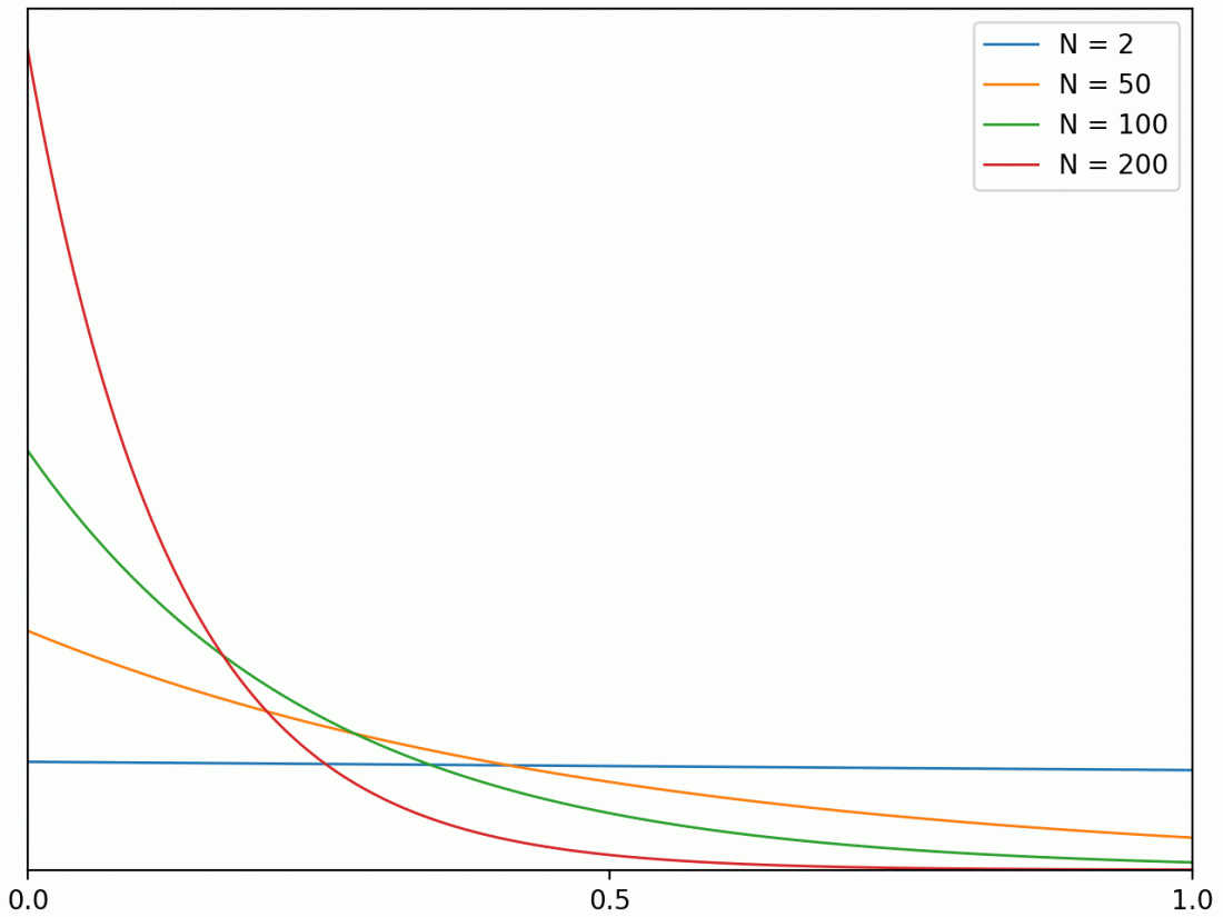
With Bose–Einstein statistics, things are drastically different. The total number of heads is uniform, regardless of how big a number of coins are used. So, for example, there will be a 20% chance of at least 90% of the coins all being the same way up. Microscopic random effects no longer average out, so these also produce random macroscopic behaviour.

Next, suppose that we have tossed a very large number N of identical coins and select them one by one, and observe if they are heads or tails. By symmetry, the first coin will be heads with probability 1/2. Then, what will be the probability of heads for the second coin, or the third, and so on? For classical coins, the probability is always 1/2, regardless of what has been observed so far. However, this independence does not hold for bosonic coins. As the proportion of heads is uniformly distributed on the unit interval, the probability of the first n being all heads is . Taking ratios then, the probability of the n’th coin being heads conditional on the first all showing heads is . For this is 1/2 as expected, but it increases to 1 as n increases. So, the more heads that we see, the greater the probability that the next one is also heads.

For more discussion of quantum coins, dice (and children!), see the 1999 article Quantum Coins, Dice and Children: Probability and Quantum Statistics by Chi-Keung Chow and Thomas D. Cohen.

---

Biased Coins

Things get even more interesting if we consider biased coins, where a single coin toss gives a head with probability . We also suppose that p is strictly between 0 and 1, otherwise it is not interesting, and set for the probability of tails. For N classical coins, the situation is very similar to the unbiased case above. The number of heads is binomially distributed, with mean and variance . Hence, dividing through by N, the proportion of heads has mean p and standard deviation , which goes to zero as N goes to infinity. As before, the randomness vanishes in the limit of large N, and we obtain a fixed proportion p of heads.

The situation is quite different for biased bosonic coins. Since, we no longer have the simple symmetry argument used above whereby all outcomes have the same probability, it is not immediately obvious what the probabilities are. Consider tossing N coins and look at the outcomes corresponding to m heads. Classically, the number of ways that this can occur is equal to the number of ways of choosing m from a collection of N objects, given by the binomial coefficient . Each of these outcomes has probability . Adding all outcomes with m heads, this gives the binomial probability . For bosonic coins, each of these possibilities should be interpreted as the same outcome, so we do not scale by the binomial coefficient, and might expect the probability to be simply . Unfortunately, this does not work. If we sum over all such ‘probabilities’, we obtain

which is strictly less than one. To fix this, we normalise the distribution by scaling with this constant, giving the probability of m heads as , which is indeed consistent with observations for bosons. For , so that tails are more likely than heads, we can write this as for a normalisation constant . This has the convenient property that, other than the constant multiplier, the probability does not depend on N and has a finite sum over m. So, as N is increased to infinity, the probability of m heads converges to a limit , with the normalisation constant . This is a geometric distribution with mean .

For biased bosonic coins with , we arrive at a very surprising result. As the total number N of coins is increased towards infinity, the number of heads converges to a finite limit. For example, if a single coin has probability 1/3 of coming up heads then, for an arbitrarily large number of coins, we would expect on average for there to be only a single head! Furthermore, the probability of there being no heads whatsoever tends to the nonzero number . If we look at the proportion of heads then, dividing through by N, we see that it tends to zero. This is shown in figure 2 below, for a value of p very close to 50% and various values of N. As above, I multiply the probabilities through by , so that they approximate probability densities. In a similar way, if p is greater than 1/2, then the proportion of heads tends to one, and we have a nonvanishing probability of all coins being heads.

This behaviour is, for example, seen in Bose–Einstein condensates and is responsible for their various strange properties, such as quantum vortices and superfluidity. All, or almost all, of the particles in the condensate tend to fall into the same low energy state.