Poisson Point Processes

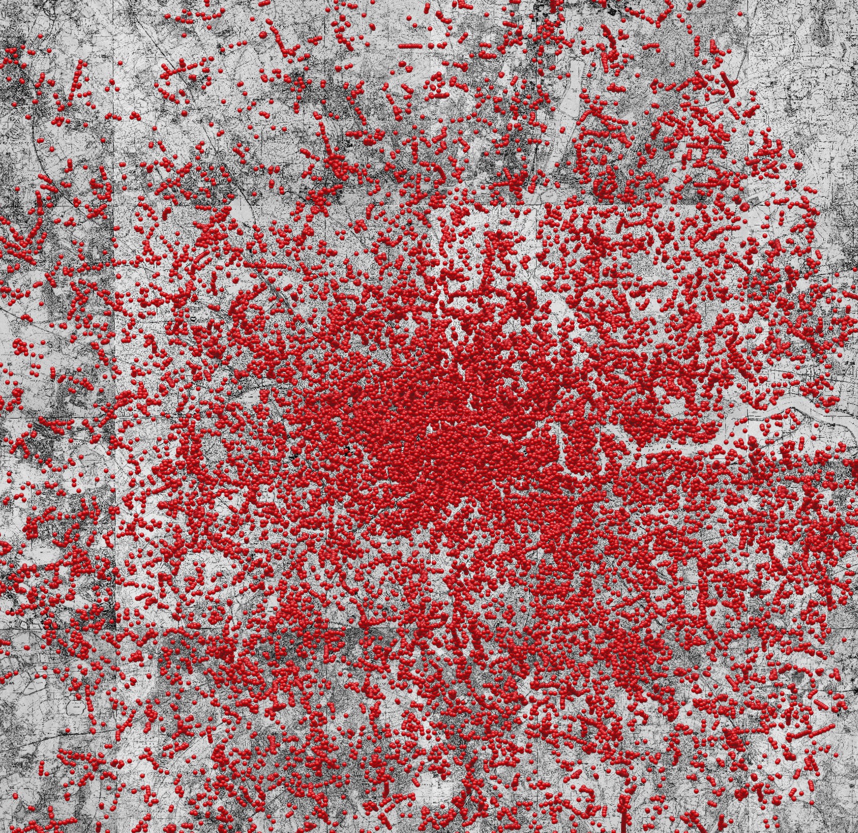
bomb map — Figure 1: Bomb map of the London Blitz, 7 October 1940 to 6 June 1941.
Obtained from http://www.bombsight.org (version 1) on 26 October 2020.

The Poisson distribution models numbers of events that occur in a specific period of time given that, at each instant, whether an event occurs or not is independent of what happens at all other times. Examples which are sometimes cited as candidates for the Poisson distribution include the number of phone calls handled by a telephone exchange on a given day, the number of decays of a radio-active material, and the number of bombs landing in a given area during the London Blitz of 1940-41. The Poisson process counts events which occur according to such distributions.

More generally, the events under consideration need not just happen at specific times, but also at specific locations in a space E. Here, E can represent an actual geometric space in which the events occur, such as the spacial distribution of bombs dropped during the Blitz shown in figure 1, but can also represent other quantities associated with the events. In this example, E could represent the 2-dimensional map of London, or could include both space and time so that ${E=F\times{\mathbb R}}$ where, now, F represents the 2-dimensional map and E is used to record both time and location of the bombs. A Poisson point process is a random set of points in E, such that the number that lie within any measurable subset is Poisson distributed. The aim of this post is to introduce Poisson point processes together with the mathematical machinery to handle such random sets.

The choice of distribution is not arbitrary. Rather, it is a result of the independence of the number of events in each region of the space which leads to the Poisson measure, much like the central limit theorem leads to the ubiquity of the normal distribution for continuous random variables and of Brownian motion for continuous stochastic processes. A random finite subset S of a reasonably ‘nice’ (standard Borel) space E is a Poisson point process so long as it satisfies the properties,

If ${A_1,\ldots,A_n}$ are pairwise-disjoint measurable subsets of E, then the sizes of ${S\cap A_1,\ldots,S\cap A_n}$ are independent.
Individual points of the space each have zero probability of being in S. That is, ${{\mathbb P}(x\in S)=0}$ for each ${x\in E}$ .

The proof of this important result will be given in a later post.

We have come across Poisson point processes previously in my stochastic calculus notes. Specifically, suppose that X is a cadlag ${{\mathbb R}^d}$ -valued stochastic process with independent increments, and which is continuous in probability. Then, the set of points ${(t,\Delta X_t)}$ over times t for which the jump ${\Delta X}$ is nonzero gives a Poisson point process on ${{\mathbb R}_+\times{\mathbb R}^d}$ . See lemma 4 of the post on processes with independent increments, which corresponds precisely to definition 5 given below.

Recall that a nonnegative integer valued random variable N has the Poisson distribution with parameter ${\lambda\in{\mathbb R}_+}$ if

$\displaystyle {\mathbb P}(N=n)=\frac{\lambda^n}{n!}e^{-\lambda}$

(1)

for all nonnegative integer n. Alternatively, this can be defined by the generating function,

$\displaystyle {\mathbb E}[x^N]=e^{-\lambda(1-x)},$

(2)

which holds for all complex x. Simply expanding out the exponentials as power series, and equating the coefficients of powers of x, gives (1). Alternatively, using ${x=e^{-t}}$ for any complex t, this can be written as

$\displaystyle {\mathbb E}[e^{-t N}]=e^{-\lambda(1-e^{-t})},$

which is the moment generating function. This distribution is denoted as ${{\rm Po}(\lambda)}$ . It will also be convenient to include the case where infinitely many events occur, so that N has the ${{\rm Po}(\infty)}$ distribution if ${{\mathbb P}(N=\infty)=1}$ . In fact, the generating function (2) still holds in this case, so long as we restrict to the range ${0\le x < 1}$ and interpret ${x^\infty}$ and ${e^{-\infty}}$ as evaluating to zero. If M and N are independent with the ${{\rm Po}(\lambda)}$ and ${{\rm Po}(\mu)}$ distributions respectively then,

$\displaystyle \begin{aligned} {\mathbb E}[x^{M+N}] &={\mathbb E}[x^M]{\mathbb E}[x^N]\\ &=e^{-\lambda(1-x)}e^{-\mu(1-x)}\\ &=e^{-(\lambda+\mu)(1-x)}, \end{aligned}$

so that ${M+N\sim{\rm Po}(\lambda+\mu)}$ .

The next ingredient for describing Poisson point processes, is that of a random point process. It is straightforward to simply assert that we have a random variable whose values are subsets of a given space E. That is, it takes values in the power set ${\mathcal P(E)}$ . However, to do probability, it is necessary to have a sigma-algebra on which the probabilities are defined and, furthermore, that this sigma-algebra is generated by reasonably simple subsets of ${\mathcal P(E)}$ . We will be concerned with finite or, at least, countable random sets and, for this, it is convenient to represent the set by its counting measure. This is a very convenient and flexible method of representing random sets, although there some technical considerations to cover first.

Given a measurable space ${(E,\mathcal E)}$ , then any subset ${S\subseteq E}$ defines a measure by

$\displaystyle \mu_S(A)=\#(S\cap A)=\sum_{x\in A}I_S(x).$

(3)

for all ${A\in\mathcal E}$ , where ${I_S(x)=1_{\{x\in S\}}}$ is the indicator function of S. This is the counting measure for the subset S. The integral of a measurable function ${f\colon E\rightarrow\bar{\mathbb R}_+}$ is simply given by its sum over S,

$\displaystyle \int fd\mu_S=\sum_{x\in S} f(x)=\sum_{x\in E}I_S(x)f(x).$

(4)

Furthermore, if S is countable and ${\mathcal E}$ separates points, then the counting measure will be sigma-finite. We generalize a bit to allow multisets, so that S can count points of E multiple times. This is necessary in order to be able to model events that can occur simultaneously. A multiset ${S\subseteq E}$ can be identified with an ‘indicator function’ ${I_S\colon E\rightarrow{\mathbb Z}_{\ge0}}$ , and is countable if ${I_S}$ has countable support. Then, for a subset ${A\subseteq E}$ , the intersection ${S\cap A}$ denotes the multiset with indicator function ${I_{S\cap A}=I_SI_A}$ , and (3) denotes the sum of ${I_S(x)}$ over ${x\in A}$ . Similarly, the summation over S in (4) is understood to be with multiplicity, so that it is equal to the sum of ${I_S(x)f(x)}$ over ${x\in E}$ . Sigma-finite measures taking only integer (or infinite) values will be referred to as point measures.

Going in the opposite direction, point measures on a reasonably nice measurable space ${(E,\mathcal E)}$ can be shown to be the counting measure associated with a unique multiset. We consider standard Borel Spaces, which are sufficient for most applications of probability and measure theory. These can be defined as measurable spaces ${(E,\mathcal E)}$ which are Borel isomorphic to a Polish space X together with its Borel sigma-algebra ${\mathcal B(X)}$ . Equivalently, there exists a complete separable metric for E with respect to which ${\mathcal E}$ is its Borel sigma-algebra. By a theorem of Kuratowski, it is known that all uncountable standard Borel spaces are isomorphic to each other. Hence, up to isomorphism, the following enumerates all standard Borel spaces.

the real numbers together with its standard Borel sigma-algebra.
the natural numbers ${{\mathbb N}}$ together with its power set.
a finite sequence ${\{1,2,\ldots,n\}}$ together with its power set, for some ${n\in{\mathbb N}}$ .

Alternatively, up to isomorphism, we can consider E to be a compact subset of the reals, together with its Borel sets. Specifically, we take ${E=[0,1]}$ in the uncountable case, ${E=\{0\}\cup\{1/n\colon n=1,2,\ldots\}}$ in the countably infinite case, and ${E=\{1/1,1/2,\ldots,1/n\}}$ in the finite case.

We obtain equivalence between countable multisets and sigma-finite measures taking values in the extended nonnegative integers ${\bar{\mathbb Z}_+=\{0,1,\ldots,\infty\}}$ .

Lemma 1 Let ${\mu}$ be a sigma-finite ${\bar{\mathbb Z}_+}$ -valued measure on Borel space ${(E,\mathcal E)}$ . Then, it is the counting measure of a unique multiset ${S\subseteq E}$ .

Proof: The uniqueness of S is immediate since, if ${\mu=\mu_S}$ then the indicator function is determined by ${I_S(x)=\mu(\{x\})}$ . Only existence of S remains to be shown.

As ${\mu}$ is a sigma-finite measure, E can be decomposed into a (finite or countably infinite) sequence of atoms ${E_n}$ ( ${1\le n < N}$ ) and a non-atomic set ${E_0}$ ,

$\displaystyle E=\bigcup_{0\le n < N}E_n.$

First, ${E_0}$ must have zero measure. If not, as the measure is integer valued, we could find ${A\subseteq E_0}$ with nonzero measure minimising ${\mu(A)}$ . This would then be an atom, contradicting the choice of ${E_0}$ . So, for any ${A\in\mathcal E}$ ,

$\displaystyle \mu(A)=\sum_{1\le n < N}\mu(E_n\cap A).$

To complete the proof, we just need to show that all atoms can be represented by singletons, so that ${E_n=\{x_n\}}$ for a pairwise distinct sequence ${x_n\in E}$ . This would give

$\displaystyle \mu(A)=\sum_{1\le n < N}1_{\{x_n\in A\}}\mu(\{x_n\})=\mu_S(A)$

where S is the multiset consisting of the points ${x_n}$ with multiplicity ${\mu(\{x_n\})}$ .

To show that every atom A is indeed given by a singleton, represent the space E as a compact subset of the reals. Then, for each positive integer n, E is contained in a finite union of intervals of the form ${(a-1/n,a+1/n)}$ and, hence, there exists ${a_n\in{\mathbb R}}$ such that ${(a_n-1/n,a_n+1/n)\cap A}$ has nonzero measure, so is equal to A up to a null set. Taking intersections of this sequence, we obtain a set B contained in each of the sets ${(a_n-1/n,a_n+1/n)}$ , so is either a singleton or is empty. By countable additivity, it is equal to A up to a null set, and hence is a singleton as required. ⬜

By lemma 1, we can use random measures to represent random sets. Use ${\mathcal M(E,\mathcal E)}$ to represent the space of measures on a measurable space ${(E,\mathcal E)}$ . This comes with a natural sigma-algebra, which is the smallest sigma-algebra making each of the maps

$\displaystyle \begin{aligned} &\mathcal M(E,\mathcal E)\rightarrow\bar{\mathbb R}_+,\\ &\mu\mapsto\mu(A) \end{aligned}$

measurable, for each fixed ${A\in\mathcal E}$ . With this definition, if we have a probability space ${(\Omega,\mathcal F,{\mathbb P})}$ then a map ${\xi\colon\Omega\rightarrow\mathcal M(E,\mathcal E)}$ is measurable if and only if ${\xi(A)}$ is a measurable random variable for all ${A\in\mathcal E}$ .

Definition 2 A random measure ${\xi}$ on a measurable space ${(E,\mathcal E)}$ , defined with respect to a probability space ${(\Omega,\mathcal F,{\mathbb P})}$ , is a measurable map

$\displaystyle \begin{aligned} &\Omega\rightarrow\mathcal M(E,\mathcal E),\\ &\omega\mapsto\xi_\omega. \end{aligned}$

such that, there exists a sequence ${A_n\in\mathcal E}$ with ${\bigcup_nA_n=E}$ and ${\xi(A_n)}$ is almost surely finite for each n.

A point process is a random measure taking values in the point measures, so that ${\xi(A)\in\bar{\mathbb Z}_+}$ for all ${A\in\mathcal E}$ .

Referring back to lemma 1, a point process ${\xi}$ on a standard Borel space ${(E,\mathcal E)}$ is uniquely expressed as the counting measure of a random multiset in E.

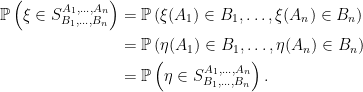
For any random measure ${\xi}$ as in definition 2, we can speak of its distribution, which is just the probability measure that it defines on the measurable subsets of ${\mathcal M(E,\mathcal E)}$ ,

$\displaystyle S\mapsto {\mathbb P}(\{\omega\in\Omega\colon\xi_\omega\in S\}).$

Given two random measures ${\xi,\eta}$ defined with respect to, possibly different, probability spaces, we write ${\xi\overset{d}{=}\eta}$ to mean that they are equal in distribution. It is a straightforward application of the pi-system lemma to show that this is equivalent to equality of their finite distributions or, in other words,

$\displaystyle \left(\xi(A_1),\ldots,\xi(A_n)\right)\overset{d}{=}\left(\eta(A_1),\ldots,\eta(A_n)\right)$

(5)

for all finite sequences ${A_1,A_2,\ldots,A_n\in\mathcal E}$ . In fact, it is sufficient to consider the case where the ${A_i}$ are pairwise disjoint.

Lemma 3 Let ${\xi,\eta}$ be random measures on a measurable space ${(E,\mathcal E)}$ . Then ${\xi\overset{d}{=}\eta}$ if and only if (5) holds for all pairwise disjoint finite sequences ${A_1,A_2,\ldots,A_n\in\mathcal E}$ .

Proof: The ‘only if’ direction is immediate from the definition of equality in distribution. Considering the ‘if’ direction, suppose that (5) holds for all pairwise disjoint sequences ${A_i\in\mathcal E}$ . Choosing a finite sequence ${A_1,\ldots,A_n}$ , we show that (5) holds, even when they are not pairwise disjoint.

Set ${A_i^1=A_i}$ , ${A_i^0=E\setminus A_i}$ and,

$\displaystyle A^\epsilon=A_1^{\epsilon_1}\cap A_2^{\epsilon_2}\cap\cdots\cap A_n^{\epsilon_n}$

for all ${\epsilon\in\{0,1\}^n}$ . These sets are pairwise disjoint so, by the condition of the lemma, ${(\xi(A^\epsilon)\colon\epsilon\in\{0,1\}^n)}$ and ${(\eta(A^\epsilon)\colon\epsilon\in\{0,1\}^n)}$ have the same distribution. Furthermore, by finite additivity of measures,

$\displaystyle \begin{aligned} A_i=\bigcup_{\epsilon\in\{0,1\}^n,\epsilon_i=1}A^\epsilon,\\ \xi(A_i)=\sum_{\epsilon\in\{0,1\}^n,\epsilon_i=1}\xi(A^\epsilon),\\ \eta(A_i)=\sum_{\epsilon\in\{0,1\}^n,\epsilon_i=1}\eta(A^\epsilon). \end{aligned}$

So, equality in distribution (5) holds as claimed.

Next, for finite sequences ${A_1,\ldots,A_n\in\mathcal E}$ and Borel measurable sets ${B_1,\ldots,B_n\subseteq\bar{\mathbb R}_+}$ , define the set

$\displaystyle S^{A_1,\ldots,A_n}_{B_1,\ldots,B_n}=\left\{\mu\in\mathcal M(E,\mathcal E)\colon\mu(A_i)\in B_i,i=1,\ldots,n\right\}.$

These form a pi-system generating the sigma-algebra on ${\mathcal M(E,\mathcal E)}$ . By equality in distribution (5),

$\displaystyle \begin{aligned} {\mathbb P}\left(\xi\in S^{A_1,\ldots,A_n}_{B_1,\ldots,B_n}\right) &={\mathbb P}\left(\xi(A_1)\in B_1,\ldots,\xi(A_n)\in B_n\right)\\ &={\mathbb P}\left(\eta(A_1)\in B_1,\ldots,\eta(A_n)\in B_n\right)\\ &={\mathbb P}\left(\eta\in S^{A_1,\ldots,A_n}_{B_1,\ldots,B_n}\right). \end{aligned}$

So, by the pi-system lemma, ${\xi}$ and ${\eta}$ have the same distribution. ⬜

It follows from this lemma that, to define the distribution of a random measure, it is sufficient to specify the distributions of ${(\xi(A_1),\ldots,\xi(A_n))}$ for pairwise disjoint finite sequences ${A_1,\ldots,A_n\in\mathcal E}$ . The independent increments property reduces this further to specifying the distribution of ${\xi(A)}$ for each ${A\in\mathcal E}$ .

Definition 4 Let ${\xi}$ be a random measure on measurable space ${(E,\mathcal E)}$ . We say that it has independent increments if, for each pairwise disjoint finite sequence ${A_1,A_2,\ldots,A_n\in\mathcal E}$ , then ${\xi(A_1),\ldots,\xi(A_n)}$ are independent random variables.

Poisson point processes are described by an intensity measure ${\mu}$ on the underlying space, which specifies the distribution of the random points contained in any measurable subset. If the underlying space is a subset of Euclidean space ${{\mathbb R}^n}$ , then intensity measures can be constructed from locally integrable density functions ${\lambda\colon E\rightarrow{\mathbb R}_+}$ ,

$\displaystyle d\mu(x)=\lambda(x)dx.$

For example, in the bomb map in figure 1, we would expect ${\lambda}$ to be peaked at the main enemy targets, around central London, and decay away as we move further out from the city.

Definition 5 Let ${(E,\mathcal E,\mu)}$ be a sigma-finite measure space. Then, a Poisson point process ${\xi}$ on ${(E,\mathcal E)}$ with intensity ${\mu}$ is a point process on ${(E,\mathcal E)}$ satisfying,

${\xi}$ has independent increments.

${\xi(A)\sim{\rm Po}(\mu(A))}$ , for each ${A\in\mathcal E}$ .

The consistency of the finite dimensional distributions follows from the fact that the sum of independent Poisson distributed random variables is itself Poisson, with parameter equal to the sum of the parameters of the random variables. That is, the sum of independent ${{\rm Po}(a)}$ and ${{\rm Po}(b)}$ distributed random variables has the ${{\rm Po}(a+b)}$ distribution. If ${A_1,\ldots,A_n}$ are pairwise disjoint measurable subsets of E so that, according to definition 5, the random variables ${\xi(A_k)}$ are independently Poisson distributed with parameters ${\mu(A_k)}$ then,

$\displaystyle \xi\left(A_1\cup\cdots\cup A_n\right)=\xi(A_1)+\cdots+\xi(A_n)$

has the Poisson distribution with parameter

$\displaystyle \mu(A_1)+\cdots+\mu(A_n)=\mu\left(A_1\cup\cdots\cup A_n\right)$

as required.

As a random variable with the ${{\rm Po}(a)}$ distribution has mean equal to ${a}$ , the intensity measure of a Poisson point process ${\xi}$ is given simply as ${\mu(A)={\mathbb E}[\xi(A)]}$ . More generally, the expectation of any random measure is itself a (non-random) measure.

Definition 6 If ${\xi}$ is a random measure on ${(E,\mathcal E)}$ , then its expected value ${\mu={\mathbb E}\xi}$ is the measure on ${(E,\mathcal E)}$ defined by

$\displaystyle \mu(A)={\mathbb E}[\xi(A)]$

for all ${A\in\mathcal E}$ .

Countable additivity of expectations and of the random measure ${\xi}$ immediately gives countable additivity for ${{\mathbb E}\xi}$ , so it is a true measure as claimed. By definition of random measures, there exists a sequence ${A_n\in\mathcal E}$ whose union covers the space E and such that ${\xi(A_n)}$ are almost-surely finite. As their expectations need not be finite, it does not follow that ${\mu}$ is sigma-finite. However, if ${\xi(A_n)}$ are Poisson distributed, then they must also have finite mean, so that ${{\mathbb E}\xi}$ is a sigma-finite measure. This shows that a point process ${\xi}$ is a Poisson point process if and only if,

${\xi}$ has independent increments.
${\xi(A)}$ has a Poisson distribution for each ${A\in\mathcal E}$ .

This definition does not require us to start from an intensity measure but, still, the intensity does exist and is given by ${\mu={\mathbb E}\xi}$ .

Existence of Poisson Point Processes

Poisson point processes corresponding to a given sigma-finite intensity measure do indeed exist, and are uniquely determined.

Theorem 7 Let ${(E,\mathcal E,\mu)}$ be a sigma-finite measure space. Then, there exists a Poisson point process on ${(E,\mathcal E)}$ with intensity ${\mu}$ , which is unique in distribution.

The proof of this result is the aim of the remainder of the post. Uniqueness follows immediately from the definition and lemma 3, so we only need to prove existence. This will be done with the help of a couple of lemmas. Recall that the sum of independent Poisson random variables is itself Poisson. The same is true of Poisson point processes, even for infinite sums.

Lemma 8 Let ${\xi_1,\xi_2,\ldots}$ be an independent sequence of Poisson point processes on a measurable space ${(E,\mathcal E)}$ , and intensity measures ${\mu_n}$ . We suppose that ${\mu=\sum_{n=1}^\infty\mu_n}$ is sigma-finite. Then, ${\xi=\sum_{n=1}^\infty\xi_n}$ is a Poisson point process with intensity ${\mu}$ .

Proof: For a pairwise disjoint sequence ${A_1,\ldots,A_m\in\mathcal E}$ , it just needs to be shown that ${\xi(A_i)}$ is a sequence of independent ${{\rm Po}(\mu(A_i))}$ distributed random variables. For this, we compute its joint generating function, which is the expected value of ${x_1^{\xi(A_1)}\cdots x_m^{\xi_m(A_m)}}$ for real ${0\le x_i < 1}$ .

$\displaystyle \begin{aligned} {\mathbb E}\left[\prod\nolimits_ix_i^{\xi(A_i)}\right] &={\mathbb E}\left[\prod\nolimits_i\prod\nolimits_nx_i^{\xi_n(A_i)}\right]\\ &=\prod\nolimits_n{\mathbb E}\left[\prod\nolimits_ix_i^{\xi_n(A_i)}\right]\\ &=\prod\nolimits_n\prod\nolimits_i{\mathbb E}\left[x_i^{\xi_n(A_i)}\right]\\ &=\prod\nolimits_n\prod\nolimits_ie^{-\mu_n(A_i)(1-x_i)}\\ &=\prod\nolimits_ie^{-\mu(A_i)(1-x_i)}\\ \end{aligned}$

This makes use of the independence of ${\xi_n}$ to extract the product over n from the expectation then, for each n, uses the independence of ${\xi_n(A_i)}$ to extract the product over i. Finally, we substituted in the moment generating function for the ${{\rm Po}(\mu_n(A_i))}$ random variable ${\xi_n(A_i)}$ . The result is the product of moment generating functions of ${{\rm Po}(\mu(A_i))}$ random variables, as required. ⬜

There is a straightforward method of constructing Poisson point processes with finite intensity measure. We start with an IID sequence of random variables ${X_1,X_2,\ldots}$ taking values in the space E. Then, consider the random multiset ${\{X_1,\ldots,X_N\}}$ , where N is Poisson independently of the ${X_i}$ .

Lemma 9 Let ${(E,\mathcal E,\mu)}$ be a probability space and ${\lambda}$ be a nonnegative real. Let N be a ${{\rm Po}(\lambda)}$ distributed random variable defined on some probability space ${(\Omega,\mathcal F,{\mathbb P})}$ and, independent of ${N}$ , let ${X_1,X_2,\ldots}$ be an IID sequence of E-valued random variables with distribution ${\mu}$ .

Then,

$\displaystyle \xi(A)=\sum_{n=1}^N1_{\{X_n\in A\}}$

for all ${A\in\mathcal E}$ , defines a Poisson point process on ${(E,\mathcal E)}$ with intensity measure ${\lambda\mu}$ , with respect to the probability space ${(\Omega,\mathcal F,{\mathbb P})}$ .

Proof: As in the proof of lemma 8, for a pairwise disjoint sequence ${A_1,\ldots,A_m\in\mathcal E}$ , it just needs to be shown that ${\xi(A_i)}$ is a sequence of independent ${{\rm Po}(\lambda\mu(A_i))}$ distributed random variables. Again, we do this by computing the joint generating function. For real numbers ${0\le x_i < 1}$ , start by taking expectations conditional on N.

$\displaystyle \begin{aligned} {\mathbb E}\left[\prod\nolimits_ix_i^{\xi(A_i)}\;\Big\vert N\right] &={\mathbb E}\left[\prod\nolimits_i\prod\nolimits_{n=1}^Nx_i^{1_{\{X_n\in A_i\}}}\;\Big\vert N\right]\\ &=\prod\nolimits_{n=1}^N{\mathbb E}\left[\prod\nolimits_i x_i^{1_{\{X_n\in A_i\}}}\;\Big\vert N\right]. \end{aligned}$

By independence of the sequence ${X_n}$ and N, the expectation conditional on N is just the same as the unconditioned expectation. Furthermore, as ${A_i}$ are pairwise disjoint, the product ${\prod_ix_i^{1_{\{X_n\in A_i\}}}}$ is equal to ${1-\sum_i1_{\{X_n\in A_i\}}(1-x_i)}$ giving,

$\displaystyle {\mathbb E}\left[\prod\nolimits_ix_i^{\xi(A_i)}\;\Big\vert N\right]=\left(1-\sum\nolimits_i\mu(A_i)(1-x_i)\right)^N.$

Taking the expectation of this and substituting in the generating function for the ${{\rm Po}(\lambda)}$ distribution for N,

$\displaystyle \begin{aligned} {\mathbb E}\left[\prod\nolimits_ix_i^{\xi(A_i)}\right] &=e^{-\lambda\sum\nolimits_i\mu(A_i)(1-x_i)}\\ &=\prod\nolimits_ie^{-\lambda\mu(A_i)(1-x_i)}. \end{aligned}$

This is the product of generating functions of ${{\rm Po}(\lambda\mu(A_i))}$ distributions, as required. ⬜

Combining the two lemmas above provides us with Poisson point measures for arbitrary sigma-finite intensity measures.

Proof of Theorem 7: Start with the case where ${(E,\mathcal E,\mu)}$ is a finite measure space. As the case where ${\lambda\equiv\mu(E)}$ is zero is trivial, we suppose that ${\lambda > 0}$ . Then, ${\nu\equiv\lambda^{-1}\mu}$ is a probability measure on ${(E,\mathcal E)}$ . By taking the product of the ${{\rm Po}(\lambda)}$ distribution on ${{\mathbb Z}_+}$ and an infinite product of ${(E,\mathcal E,\nu)}$ , we obtain a probability space ${(\Omega,\mathcal F,{\mathbb P})}$ on which there are defined a ${{\rm Po}(\lambda)}$ random variable N and, independently, an IID sequence ${X_1,X_2,\ldots}$ of E-valued random variables with distribution ${\nu}$ . Lemma 9 then provides us with a Poisson point process with intensity ${\mu=\lambda\nu}$ .

Now, suppose that ${\mu}$ is a sigma-finite measure. Then, we can write ${\mu=\sum_{n=1}^\infty\mu_n}$ for finite measures ${\mu_n}$ on ${(E,\mathcal E)}$ . By what we have shown above, there exists Poisson point processes ${\xi_n}$ with intensity ${\mu_n}$ , possibly defined with respect to different probability spaces. Taking the product over n of these probability spaces, we can suppose that ${\xi_n}$ are all defined with respect the same probability space and are independent. Lemma 8 says that ${\xi=\sum_{n=1}^\infty\xi_n}$ is a Poisson point process with intensity ${\mu}$ . ⬜

	Harry on Filtrations and Adapted P…
	Anonymous on Analytic Sets
	Daniel on Analytic Sets
	Sid on Martingale Convergence
	northwiz on Preservation of the Local Mart…
	George Lowther on Martingale Convergence
	Sid on Martingale Convergence
	George Lowther on The Burkholder-Davis-Gundy Ine…
	George Lowther on Preservation of the Local Mart…
	northwiz on Preservation of the Local Mart…

Poisson Point Processes

Existence of Poisson Point Processes

Published by George Lowther

Leave a Reply Cancel reply

Existence of Poisson Point Processes

Like this:

Related

Published by George Lowther

Leave a Reply Cancel reply