Criteria for Poisson Point Processes

If S is a finite random set in a standard Borel measurable space ${(E,\mathcal E)}$ satisfying the following two properties,

if ${A,B\in\mathcal E}$ are disjoint, then the sizes of ${S\cap A}$ and ${S\cap B}$ are independent random variables,
${{\mathbb P}(x\in S)=0}$ for each ${x\in E}$ ,

then it is a Poisson point process. That is, the size of ${S\cap A}$ is a Poisson random variable for each ${A\in\mathcal E}$ . This justifies the use of Poisson point processes in many different areas of probability and stochastic calculus, and provides a convenient method of showing that point processes are indeed Poisson. If the theorem applies, so that we have a Poisson point process, then we just need to compute the intensity measure to fully determine its distribution. The result above was mentioned in the previous post, but I give a precise statement and proof here. Continue reading “Criteria for Poisson Point Processes” →

Poisson Point Processes

bomb map — Figure 1: Bomb map of the London Blitz, 7 October 1940 to 6 June 1941.
Obtained from http://www.bombsight.org (version 1) on 26 October 2020.

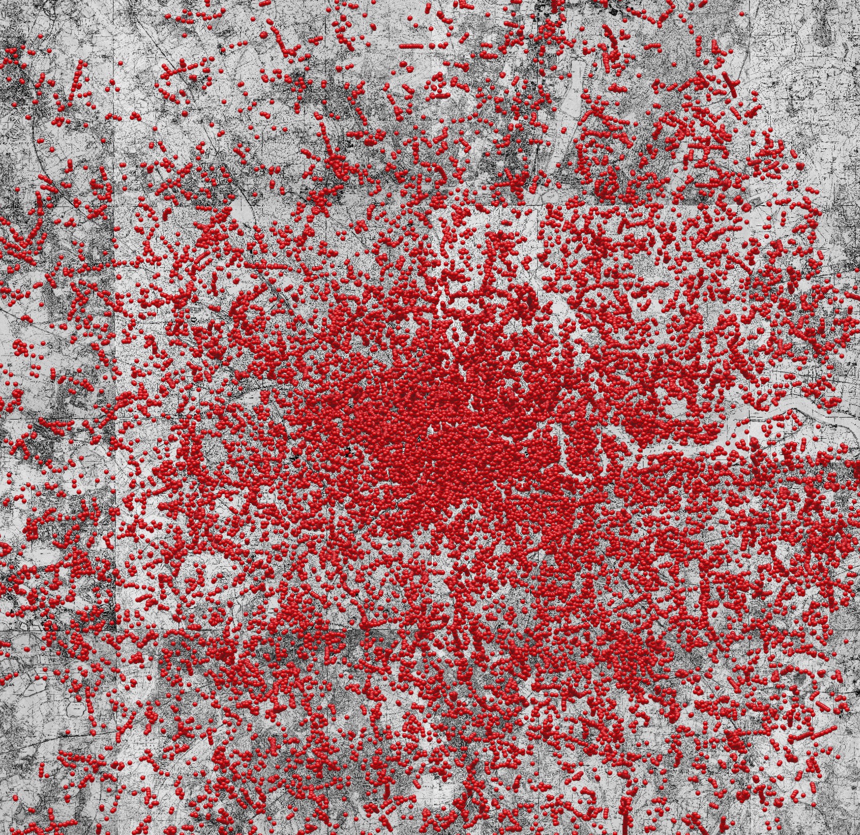
The Poisson distribution models numbers of events that occur in a specific period of time given that, at each instant, whether an event occurs or not is independent of what happens at all other times. Examples which are sometimes cited as candidates for the Poisson distribution include the number of phone calls handled by a telephone exchange on a given day, the number of decays of a radio-active material, and the number of bombs landing in a given area during the London Blitz of 1940-41. The Poisson process counts events which occur according to such distributions.

More generally, the events under consideration need not just happen at specific times, but also at specific locations in a space E. Here, E can represent an actual geometric space in which the events occur, such as the spacial distribution of bombs dropped during the Blitz shown in figure 1, but can also represent other quantities associated with the events. In this example, E could represent the 2-dimensional map of London, or could include both space and time so that ${E=F\times{\mathbb R}}$ where, now, F represents the 2-dimensional map and E is used to record both time and location of the bombs. A Poisson point process is a random set of points in E, such that the number that lie within any measurable subset is Poisson distributed. The aim of this post is to introduce Poisson point processes together with the mathematical machinery to handle such random sets.

The choice of distribution is not arbitrary. Rather, it is a result of the independence of the number of events in each region of the space which leads to the Poisson measure, much like the central limit theorem leads to the ubiquity of the normal distribution for continuous random variables and of Brownian motion for continuous stochastic processes. A random finite subset S of a reasonably ‘nice’ (standard Borel) space E is a Poisson point process so long as it satisfies the properties,

If ${A_1,\ldots,A_n}$ are pairwise-disjoint measurable subsets of E, then the sizes of ${S\cap A_1,\ldots,S\cap A_n}$ are independent.
Individual points of the space each have zero probability of being in S. That is, ${{\mathbb P}(x\in S)=0}$ for each ${x\in E}$ .

The proof of this important result will be given in a later post.

We have come across Poisson point processes previously in my stochastic calculus notes. Specifically, suppose that X is a cadlag ${{\mathbb R}^d}$ -valued stochastic process with independent increments, and which is continuous in probability. Then, the set of points ${(t,\Delta X_t)}$ over times t for which the jump ${\Delta X}$ is nonzero gives a Poisson point process on ${{\mathbb R}_+\times{\mathbb R}^d}$ . See lemma 4 of the post on processes with independent increments, which corresponds precisely to definition 5 given below. Continue reading “Poisson Point Processes” →

Compensators of Counting Processes

A counting process, X, is defined to be an adapted stochastic process starting from zero which is piecewise constant and right-continuous with jumps of size 1. That is, letting ${\tau_n}$ be the first time at which ${X_t=n}$ , then

$\displaystyle X_t=\sum_{n=1}^\infty 1_{\{\tau_n\le t\}}.$

By the debut theorem, ${\tau_n}$ are stopping times. So, X is an increasing integer valued process counting the arrivals of the stopping times ${\tau_n}$ . A basic example of a counting process is the Poisson process, for which ${X_t-X_s}$ has a Poisson distribution independently of ${\mathcal{F}_s}$ , for all times ${t > s}$ , and for which the gaps ${\tau_n-\tau_{n-1}}$ between the stopping times are independent exponentially distributed random variables. As we will see, although Poisson processes are just one specific example, every quasi-left-continuous counting process can actually be reduced to the case of a Poisson process by a time change. As always, we work with respect to a complete filtered probability space ${(\Omega,\mathcal{F},\{\mathcal{F}_t\}_{t\ge0},{\mathbb P})}$ .

Note that, as a counting process X has jumps bounded by 1, it is locally integrable and, hence, the compensator A of X exists. This is the unique right-continuous predictable and increasing process with ${A_0=0}$ such that ${X-A}$ is a local martingale. For example, if X is a Poisson process of rate ${\lambda}$ , then the compensated Poisson process ${X_t-\lambda t}$ is a martingale. So, the compensator of X is the continuous process ${A_t=\lambda t}$ . More generally, X is said to be quasi-left-continuous if ${{\mathbb P}(\Delta X_\tau=0)=1}$ for all predictable stopping times ${\tau}$ , which is equivalent to the compensator of X being almost surely continuous. Another simple example of a counting process is ${X=1_{[\tau,\infty)}}$ for a stopping time ${\tau > 0}$ , in which case the compensator of X is just the same thing as the compensator of ${\tau}$ .

As I will show in this post, compensators of quasi-left-continuous counting processes have many parallels with the quadratic variation of continuous local martingales. For example, Lévy’s characterization states that a local martingale X starting from zero is standard Brownian motion if and only if its quadratic variation is ${[X]_t=t}$ . Similarly, as we show below, a counting process is a homogeneous Poisson process of rate ${\lambda}$ if and only if its compensator is ${A_t=\lambda t}$ . It was also shown previously in these notes that a continuous local martingale X has a finite limit ${X_\infty=\lim_{t\rightarrow\infty}X_t}$ if and only if ${[X]_\infty}$ is finite. Similarly, a counting process X has finite value ${X_\infty}$ at infinity if and only if the same is true of its compensator. Another property of a continuous local martingale X is that it is constant over all intervals on which its quadratic variation is constant. Similarly, a counting process X is constant over any interval on which its compensator is constant. Finally, it is known that every continuous local martingale is simply a continuous time change of standard Brownian motion. In the main result of this post (Theorem 5), we show that a similar statement holds for counting processes. That is, every quasi-left-continuous counting process is a continuous time change of a Poisson process of rate 1. Continue reading “Compensators of Counting Processes” →

Properties of Lévy Processes

Lévy processes, which are defined as having stationary and independent increments, were introduced in the previous post. It was seen that the distribution of a d-dimensional Lévy process X is determined by the characteristics ${(\Sigma,b,\nu)}$ via the Lévy-Khintchine formula,

$\displaystyle \setlength\arraycolsep{2pt} \begin{array}{rl} &\displaystyle{\mathbb E}\left[e^{ia\cdot (X_t-X_0)}\right] = \exp(t\psi(a)),\smallskip\\ &\displaystyle\psi(a)=ia\cdot b-\frac12a^{\rm T}\Sigma a+\int_{{\mathbb R}^d}\left(e^{ia\cdot x}-1-\frac{ia\cdot x}{1+\Vert x\Vert}\right)\,d\nu(x). \end{array}$

(1)

The positive semidefinite matrix ${\Sigma}$ describes the Brownian motion component of X, b is a drift term, and ${\nu}$ is a measure on ${{\mathbb R}^d}$ such that ${\nu(A)}$ is the rate at which jumps ${\Delta X\in A}$ of X occur. Then, equation (1) gives us the characteristic function of the increments of the process.

In the current post, I will investigate some of the properties of such processes, and how they are related to the characteristics. In particular, we will be concerned with pathwise properties of X. It is known that Brownian motion and Cauchy processes have infinite variation in every nonempty time interval, whereas other Lévy processes — such as the Poisson process — are piecewise constant, only jumping at a discrete set of times. There are also purely discontinuous Lévy processes which have infinitely many discontinuities, yet are of finite variation, on every interval (e.g., the gamma process). Continue reading “Properties of Lévy Processes” →

Lévy Processes

A Poisson process sample path — Figure 1: A Cauchy process sample path

Continuous-time stochastic processes with stationary independent increments are known as Lévy processes. In the previous post, it was seen that processes with independent increments are described by three terms — the covariance structure of the Brownian motion component, a drift term, and a measure describing the rate at which jumps occur. Being a special case of independent increments processes, the situation with Lévy processes is similar. However, stationarity of the increments does simplify things a bit. We start with the definition.

Definition 1 (Lévy process) A d-dimensional Lévy process X is a stochastic process taking values in ${{\mathbb R}^d}$ such that

independent increments: ${X_t-X_s}$ is independent of ${\{X_u\colon u\le s\}}$ for any ${s<t}$ .

stationary increments: ${X_{s+t}-X_s}$ has the same distribution as ${X_t-X_0}$ for any ${s,t>0}$ .

continuity in probability: ${X_s\rightarrow X_t}$ in probability as s tends to t.

More generally, it is possible to define the notion of a Lévy process with respect to a given filtered probability space ${(\Omega,\mathcal{F},\{\mathcal{F}_t\}_{t\ge0},{\mathbb P})}$ . In that case, we also require that X is adapted to the filtration and that ${X_t-X_s}$ is independent of ${\mathcal{F}_s}$ for all ${s < t}$ . In particular, if X is a Lévy process according to definition 1 then it is also a Lévy process with respect to its natural filtration ${\mathcal{F}_t=\sigma(X_s\colon s\le t)}$ . Note that slightly different definitions are sometimes used by different authors. It is often required that ${X_0}$ is zero and that X has cadlag sample paths. These are minor points and, as will be shown, any process satisfying the definition above will admit a cadlag modification.

The most common example of a Lévy process is Brownian motion, where ${X_t-X_s}$ is normally distributed with zero mean and variance ${t-s}$ independently of ${\mathcal{F}_s}$ . Other examples include Poisson processes, compound Poisson processes, the Cauchy process, gamma processes and the variance gamma process.

For example, the symmetric Cauchy distribution on the real numbers with scale parameter ${\gamma > 0}$ has probability density function p and characteristic function ${\phi}$ given by,

$\displaystyle \setlength\arraycolsep{2pt} \begin{array}{rl} &\displaystyle p(x)=\frac{\gamma}{\pi(\gamma^2+x^2)},\smallskip\\ &\displaystyle\phi(a)\equiv{\mathbb E}\left[e^{iaX}\right]=e^{-\gamma\vert a\vert}. \end{array}$

(1)

From the characteristic function it can be seen that if X and Y are independent Cauchy random variables with scale parameters ${\gamma_1}$ and ${\gamma_2}$ respectively then ${X+Y}$ is Cauchy with parameter ${\gamma_1+\gamma_2}$ . We can therefore consistently define a stochastic process ${X_t}$ such that ${X_t-X_s}$ has the symmetric Cauchy distribution with parameter ${t-s}$ independent of ${\{X_u\colon u\le t\}}$ , for any ${s < t}$ . This is called a Cauchy process, which is a purely discontinuous Lévy process. See Figure 1.

Lévy processes are determined by the triple ${(\Sigma,b,\nu)}$ , where ${\Sigma}$ describes the covariance structure of the Brownian motion component, b is the drift component, and ${\nu}$ describes the rate at which jumps occur. The distribution of the process is given by the Lévy-Khintchine formula, equation (3) below.

Theorem 2 (Lévy-Khintchine) Let X be a d-dimensional Lévy process. Then, there is a unique function ${\psi\colon{\mathbb R}\rightarrow{\mathbb C}}$ such that

$\displaystyle {\mathbb E}\left[e^{ia\cdot (X_t-X_0)}\right]=e^{t\psi(a)}$ (2)

for all ${a\in{\mathbb R}^d}$ and ${t\ge0}$ . Also, ${\psi(a)}$ can be written as

$\displaystyle \psi(a)=ia\cdot b-\frac{1}{2}a^{\rm T}\Sigma a+\int _{{\mathbb R}^d}\left(e^{ia\cdot x}-1-\frac{ia\cdot x}{1+\Vert x\Vert}\right)\,d\nu(x)$ (3)

where ${\Sigma}$ , b and ${\nu}$ are uniquely determined and satisfy the following,

${\Sigma\in{\mathbb R}^{d^2}}$ is a positive semidefinite matrix.

${b\in{\mathbb R}^d}$ .

${\nu}$ is a Borel measure on ${{\mathbb R}^d}$ with ${\nu(\{0\})=0}$ and,

$\displaystyle \int_{{\mathbb R}^d}\Vert x\Vert^2\wedge 1\,d\nu(x)<\infty.$ (4)

Furthermore, ${(\Sigma,b,\nu)}$ uniquely determine all finite distributions of the process ${X-X_0}$ .

Conversely, if ${(\Sigma,b,\nu)}$ is any triple satisfying the three conditions above, then there exists a Lévy process satisfying (2,3).

Continue reading “Lévy Processes” →

Processes with Independent Increments

In a previous post, it was seen that all continuous processes with independent increments are Gaussian. We move on now to look at a much more general class of independent increments processes which need not have continuous sample paths. Such processes can be completely described by their jump intensities, a Brownian term, and a deterministic drift component. However, this class of processes is large enough to capture the kinds of behaviour that occur for more general jump-diffusion processes. An important subclass is that of Lévy processes, which have independent and stationary increments. Lévy processes will be looked at in more detail in the following post, and includes as special cases, the Cauchy process, gamma processes, the variance gamma process, Poisson processes, compound Poisson processes and Brownian motion.

Recall that a process ${\{X_t\}_{t\ge0}}$ has the independent increments property if ${X_t-X_s}$ is independent of ${\{X_u\colon u\le s\}}$ for all times ${0\le s\le t}$ . More generally, we say that X has the independent increments property with respect to an underlying filtered probability space ${(\Omega,\mathcal{F},\{\mathcal{F}_t\}_{t\ge0},{\mathbb P})}$ if it is adapted and ${X_t-X_s}$ is independent of ${\mathcal{F}_s}$ for all ${s < t}$ . In particular, every process with independent increments also satisfies the independent increments property with respect to its natural filtration. Throughout this post, I will assume the existence of such a filtered probability space, and the independent increments property will be understood to be with regard to this space.

The process X is said to be continuous in probability if ${X_s\rightarrow X_t}$ in probability as s tends to t. As we now state, a d-dimensional independent increments process X is uniquely specified by a triple ${(\Sigma,b,\mu)}$ where ${\mu}$ is a measure describing the jumps of X, ${\Sigma}$ determines the covariance structure of the Brownian motion component of X, and b is an additional deterministic drift term.

Theorem 1 Let X be an ${{\mathbb R}^d}$ -valued process with independent increments and continuous in probability. Then, there is a unique continuous function ${{\mathbb R}^d\times{\mathbb R}_+\rightarrow{\mathbb C}}$ , ${(a,t)\mapsto\psi_t(a)}$ such that ${\psi_0(a)=0}$ and

$\displaystyle {\mathbb E}\left[e^{ia\cdot (X_t-X_0)}\right]=e^{i\psi_t(a)}$ (1)

for all ${a\in{\mathbb R}^d}$ and ${t\ge0}$ . Also, ${\psi_t(a)}$ can be written as

$\displaystyle \psi_t(a)=ia\cdot b_t-\frac{1}{2}a^{\rm T}\Sigma_t a+\int _{{\mathbb R}^d\times[0,t]}\left(e^{ia\cdot x}-1-\frac{ia\cdot x}{1+\Vert x\Vert}\right)\,d\mu(x,s)$ (2)

where ${\Sigma_t}$ , ${b_t}$ and ${\mu}$ are uniquely determined and satisfy the following,

${t\mapsto\Sigma_t}$ is a continuous function from ${{\mathbb R}_+}$ to ${{\mathbb R}^{d^2}}$ such that ${\Sigma_0=0}$ and ${\Sigma_t-\Sigma_s}$ is positive semidefinite for all ${t\ge s}$ .

${t\mapsto b_t}$ is a continuous function from ${{\mathbb R}_+}$ to ${{\mathbb R}^d}$ , with ${b_0=0}$ .

${\mu}$ is a Borel measure on ${{\mathbb R}^d\times{\mathbb R}_+}$ with ${\mu(\{0\}\times{\mathbb R}_+)=0}$ , ${\mu({\mathbb R}^d\times\{t\})=0}$ for all ${t\ge 0}$ and,

$\displaystyle \int_{{\mathbb R}^d\times[0,t]}\Vert x\Vert^2\wedge 1\,d\mu(x,s)<\infty.$ (3)

Furthermore, ${(\Sigma,b,\mu)}$ uniquely determine all finite distributions of the process ${X-X_0}$ .

Conversely, if ${(\Sigma,b,\mu)}$ is any triple satisfying the three conditions above, then there exists a process with independent increments satisfying (1,2).

Continue reading “Processes with Independent Increments” →

Poisson Processes

A Poisson process is a continuous-time stochastic process which counts the arrival of randomly occurring events. Commonly cited examples which can be modeled by a Poisson process include radioactive decay of atoms and telephone calls arriving at an exchange, in which the number of events occurring in each consecutive time interval are assumed to be independent. Being piecewise constant, Poisson processes have very simple pathwise properties. However, they are very important to the study of stochastic calculus and, together with Brownian motion, forms one of the building blocks for the much more general class of Lévy processes. I will describe some of their properties in this post.

A random variable N has the Poisson distribution with parameter ${\lambda}$ , denoted by ${N\sim{\rm Po}(\lambda)}$ , if it takes values in the set of nonnegative integers and

$\displaystyle {\mathbb P}(N=n)=\frac{\lambda^n}{n!}e^{-\lambda}$

(1)

for each ${n\in{\mathbb Z}_+}$ . The mean and variance of N are both equal to ${\lambda}$ , and the moment generating function can be calculated,

$\displaystyle {\mathbb E}\left[e^{aN}\right] = \exp\left(\lambda(e^a-1)\right),$

which is valid for all ${a\in{\mathbb C}}$ . From this, it can be seen that the sum of independent Poisson random variables with parameters ${\lambda}$ and ${\mu}$ is again Poisson with parameter ${\lambda+\mu}$ . The Poisson distribution occurs as a limit of binomial distributions. The binomial distribution with success probability p and m trials, denoted by ${{\rm Bin}(m,p)}$ , is the sum of m independent ${\{0,1\}}$ -valued random variables each with probability p of being 1. Explicitly, if ${N\sim{\rm Bin}(m,p)}$ then

$\displaystyle {\mathbb P}(N=n)=\frac{m!}{n!(m-n)!}p^n(1-p)^{m-n}.$

In the limit as ${m\rightarrow\infty}$ and ${p\rightarrow 0}$ such that ${mp\rightarrow\lambda}$ , it can be verified that this tends to the Poisson distribution (1) with parameter ${\lambda}$ .

Poisson processes are then defined as processes with independent increments and Poisson distributed marginals, as follows.

Definition 1 A Poisson process X of rate ${\lambda\ge0}$ is a cadlag process with ${X_0=0}$ and ${X_t-X_s\sim{\rm Po}(\lambda(t-s))}$ independently of ${\{X_u\colon u\le s\}}$ for all ${s\le t}$ .

An immediate consequence of this definition is that, if X and Y are independent Poisson processes of rates ${\lambda}$ and ${\mu}$ respectively, then their sum ${X+Y}$ is also Poisson with rate ${\lambda+\mu}$ . Continue reading “Poisson Processes” →

	Tavin on Class (D) Processes
	George Lowther on Filtrations and Adapted P…
	faceet on Filtrations and Adapted P…
	George Lowther on Filtrations and Adapted P…
	facet on Filtrations and Adapted P…
	Zoltan on Class (D) Processes
	Zoltan on Class (D) Processes
	ARS on Stopping Times and the Debut…
	George Lowther on Upcrossings, Downcrossings, an…
	George Lowther on Stopping Times and the Debut…

Like this:

Like this:

Like this:

Like this:

Like this:

Like this:

Like this: