Criteria for Poisson Point Processes

If S is a finite random set in a standard Borel measurable space ${(E,\mathcal E)}$ satisfying the following two properties,

if ${A,B\in\mathcal E}$ are disjoint, then the sizes of ${S\cap A}$ and ${S\cap B}$ are independent random variables,
${{\mathbb P}(x\in S)=0}$ for each ${x\in E}$ ,

then it is a Poisson point process. That is, the size of ${S\cap A}$ is a Poisson random variable for each ${A\in\mathcal E}$ . This justifies the use of Poisson point processes in many different areas of probability and stochastic calculus, and provides a convenient method of showing that point processes are indeed Poisson. If the theorem applies, so that we have a Poisson point process, then we just need to compute the intensity measure to fully determine its distribution. The result above was mentioned in the previous post, but I give a precise statement and proof here.

As described in the previous post, a convenient way to represent such random sets is via their counting measure, which is a measurable map from the underlying probability space to the space ${\mathcal M(E,\mathcal E)}$ of measures on the space ${(E,\mathcal E)}$ . This counts the (random) number of points of S lying in each measurable set. Use ${\xi}$ to denote this map, or point process,

$\displaystyle \xi(A)=\#(S\cap A).$

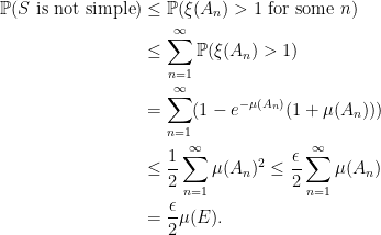
As we showed, all such integer values random measures, or point processes, describe a random set. We allow the set S to be infinite, although the definition used for random measures does require there to be a countable sequence ${A_n\in\mathcal E}$ covering E such that ${\xi(A_n)}$ are almost surely finite. Also, the point process definition does allow S to be a multiset, so that individual points in E may have a multiplicity greater than one. We will say that ${\xi}$ is a simple point process if, with probability one, the points of S each have multiplicity 1, meaning that it is a true random subset of E. Poisson point processes are always simple, so long as the intensity measure has no atoms. That is, ${{\mathbb E}\xi(\{x\})=0}$ for all ${x\in E}$ .

Lemma 1 Let ${\xi}$ be a Poisson point process on Borel space ${(E,\mathcal E)}$ . Then, ${\xi}$ is simple if and only if ${\xi(\{x\})=0}$ almost surely for each ${x\in E}$ .

Proof: The ‘only if’ direction is immediate since, if ${\xi(\{x\})}$ was nonzero with positive probability then it would have a ${{\rm Po}(\lambda)}$ distribution for some ${\lambda > 0}$ , so is greater than one with positive probability and, hence, ${\xi}$ is not simple.

For the ‘if’ direction, we suppose that ${\xi(\{x\})=0}$ almost surely for each ${x\in E}$ and need to show that the process is simple. Let us start with the case where the intensity measure ${\mu={\mathbb E}\xi}$ is finite. As ${\mu(\{x\})=0}$ for all ${x\in E}$ , it is standard that for each ${\epsilon > 0}$ , we can find a pairwise disjoint sequence ${A_1,A_2,\ldots\in\mathcal E}$ each with measure less than ${\epsilon}$ , and whose union covers E. Letting ${S\subseteq E}$ be the random multiset associated with the process, note that if S contained any point ${x}$ with multiplicity greater than 1, then ${x\in A_n}$ for some n. Hence, ${\xi(A_n)}$ would be greater than 1. So,

$\displaystyle \begin{aligned} {\mathbb P}(S{\rm\ is\ not\ simple}) &\le{\mathbb P}(\xi(A_n) > 1{\rm\ for\ some\ }n)\\ &\le\sum_{n=1}^\infty{\mathbb P}(\xi(A_n) > 1)\\ &=\sum_{n=1}^\infty(1-e^{-\mu(A_n)}(1+\mu(A_n)))\\ &\le\frac12\sum_{n=1}^\infty\mu(A_n)^2 \le\frac\epsilon2\sum_{n=1}^\infty\mu(A_n)\\ &=\frac\epsilon2\mu(E). \end{aligned}$

Taking ${\epsilon}$ arbitrarily small shows that S is almost surely simple. For the case where ${\mu}$ is sigma-finite, choose a pairwise disjoint sequence ${E_n\in\mathcal E}$ with finite measure and whose union covers E. Then, the point measures ${\xi_n(A)\equiv\xi(E_n\cap A)}$ are Poisson with finite intensity ${\mu(E_n)}$ , so are simple. If S is the random multiset associated with ${\xi}$ then, ${S\cap E_n}$ is the random multiset associated with ${\xi_n}$ and, hence, is simple. So, ${S=\bigcup_n(S\cap E_n)}$ is a union of pairwise disjoint sets, and is a true set. ⬜

I now give the main result of the post, which includes a precise statement of the criteria for Poisson point processes. It actually contains two distinct criteria, both of which are sufficient to guarantee that the process is Poisson. Firstly, there is the independent increments property. In fact, it is sufficient for pairwise independence to hold. This means that, for any pair of disjoint sets ${A,B\in\mathcal E}$ , then ${\xi(A)}$ and ${\xi(B)}$ are independent. If this holds, so that the theorem guarantees that we have a Poisson point process, then the more general independent increments property for arbitrary finite and pairwise disjoint sequences ${A_1,\ldots,A_n\in\mathcal E}$ also automatically holds. Secondly, the property that each ${\xi(A)}$ is Poisson is also sufficient, without requiring anything about the joint distributions. Recall the definition of Poisson point processes, which requires both independent increments and that ${\xi(A)}$ is Poisson for all ${A\in\mathcal E}$ . In the case that the process is simple and assigns zero value, with probability one, to each fixed point ${x\in E}$ , then either of the two defining properties are sufficient on their own.

Theorem 2 Let ${\xi}$ be a simple point process on a standard Borel space ${(E,\mathcal E)}$ such that ${\xi(\{x\})=0}$ almost surely, for each ${x\in E}$ . Then, the following are equivalent,

${\xi}$ has pairwise independent increments.

${\xi(A)}$ has a Poisson distribution for each ${A\in\mathcal E}$ .

${\xi}$ is a Poisson point process.

The proof will be given further down, with theorem 8 giving the equivalence of 1 and 3, and theorem 10 giving equivalence of 2 and 3. For now, I will look at how it applies in a simple example. Considering the values of a cadlag stochastic process at all of its jump times naturally gives rise to a point process.

Lemma 3 Let ${\{X_t\}_{t\ge0}}$ be a cadlag stochastic process taking values in separable metric space E. Then, the random set

$\displaystyle S_1=\left\{(t,X_{t-},X_t)\colon t > 0, X_{t-}\not=X_t\right\}$

defines a simple point process on ${({\mathbb R}_+\times E^2,\mathcal B({\mathbb R}_+\times E^2))}$ . If ${E={\mathbb R}^d}$ then,

$\displaystyle S_2=\left\{(t,\Delta X_t)\colon t > 0, X_{t-}\not=X_t\right\}$

also defines a simple point process, on ${({\mathbb R}_+\times{\mathbb R}^d,\mathcal B({\mathbb R}_+\times{\mathbb R}^d))}$ .

Proof: Simplicity is immediate in both cases, sice there cannot be more than one jump at the same time. Letting ${\xi}$ be the counting measure of set ${S_1}$ , it needs to shown that this is measurable and that ${\xi(A_n)}$ is finite for some sequence ${A_n}$ of measurable sets whose union is all of ${{\mathbb R}_+\times E^2}$ . Note first that, by construction, the set ${S_1}$ is disjoint from ${{\mathbb R}_+\times\Delta}$ , where ${\Delta=\{(x,x)\colon x\in E\}}$ is the diagonal. This means that ${\xi({\mathbb R}_+\times\Delta)}$ is zero, so we only need to consider sets disjoint from this. Really, we could have excluded ${{\mathbb R}_+\times\Delta}$ from the space to start with.

Letting ${d}$ be the metric for E, choose a sequence ${\epsilon_n > 0}$ tending to zero and times ${T_n}$ tending to infinity, then set

$\displaystyle A_n=\left\{(t,x,y)\in{\mathbb R}_+\times E^2\colon t < T_n, d(x,y) > \epsilon_n\right\}.$

By the cadlag property, ${A_n\cap S_1}$ is finite as required. Suppose that this was false, then there would exist an infinite sequence of distinct times ${t_m}$ such that ${(t_m,X_{t_m-},X_{t_m})}$ are all in ${A_n}$ . Passing to a subsequence if necessary, we can suppose that ${t_m}$ is monotonic and, hence, ${X_{t_m-}}$ and ${X_{t_m}}$ both tend to the same limit (either ${X_{t-}}$ or ${X_t}$ where ${t=\lim t_m}$ ), which contradicts the inequality ${d(X_{t_m-},X_{t_m}) > \epsilon}$ .

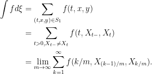
Next, consider any continuous function ${f\colon{\mathbb R}_+\times E^2\rightarrow{\mathbb R}}$ supported on one of the sets ${A_n}$ . Then,

$\displaystyle \begin{aligned} \int fd\xi &=\sum_{(t,x,y)\in S_1}f(t,x,y)\\ &=\sum_{t > 0,X_{t-}\not=X_t}f(t,X_{t-},X_t)\\ &=\lim_{m\rightarrow\infty}\sum_{k=1}^\infty f(k/m,X_{(k-1)/m},X_{k/m}). \end{aligned}$

To see why this limit holds, consider the terms inside the sum and a fixed time t such that ${(t,X_{t-},X_t)}$ is in ${A_n}$ . If, for each m, we choose k so that ${(k-1)/m < t\le k/m}$ then, ${(k/m,X_{(k-1)/m},X_{k/m})}$ tends to ${(t,X_{t-},X_t)}$ and, by continuity, the corresponding term in the sum tends to ${f(t,X_{t-},X_t)}$ . On the other hand, by continuity and the fact that ${f}$ is supported on ${A_n}$ , all of the other terms in the sum are zero for sufficiently large m.

As a limit of measurable random variables, we see that ${\int f d\xi}$ is measurable. This is where separability of E is required, to ensure that the sigma algebras ${\mathcal B({\mathbb R}_+\times E^2)}$ and ${\mathcal B({\mathbb R}_+)\otimes\mathcal B(E)\otimes\mathcal B(E)}$ are the same, so continuity of ${f}$ guarantees that ${f(t,X_{t-},X_t)}$ is a measurable random variable. Then, by the functional monotone class theorem, ${\int f d\xi}$ is measurable for any bounded measurable ${f\colon{\mathbb R}_+\times E^2\rightarrow{\mathbb R}}$ . Hence, if ${A\in\mathcal B({\mathbb R}_+\times E^2)}$ then,

$\displaystyle \mu(A)=\lim_{n\rightarrow\infty}\mu(A_n\cap A)=\lim_{n\rightarrow\infty}\int 1_{A_n\cap A}d\xi$

is a limit of measurable random variables, so is measurable.

Next, consider the case where ${E={\mathbb R}^d}$ . Use the standard Euclidean metric on E, and let ${\eta}$ be the counting measure of ${S_2}$ . Defining

$\displaystyle \begin{aligned} &\theta\colon{\mathbb R}_+\times({\mathbb R}^d)^2\rightarrow{\mathbb R}_+\times{\mathbb R}^d\\ &(t,x,y)\mapsto(t,y-x), \end{aligned}$

then ${\eta(A)=\xi(\theta^{-1}(A))}$ is measurable for all ${A\in\mathcal B({\mathbb R}_+\times{\mathbb R}^d)}$ . If we let ${B_n}$ consist of ${(t,x)\in{\mathbb R}_+\times{\mathbb R}}$ such that ${t < T_n}$ and ${\lVert x\rVert > \epsilon_n}$ , then ${\eta(B_n)=\xi(A_n)}$ is finite, showing that ${\eta}$ is a point process. ⬜

In the context of lemma 3, where we have processes evolving through time, it is natural to consider point processes on both time and space. The measurable space on which it is defined is then of the form ${{\mathbb R}_+\times E}$ , with ${{\mathbb R}_+}$ representing the time index and E representing space. Fundamentally, this is no different from the general case of a point process on a space E, we simply consider both time and space together as a single product space. It can be though of, though, as a point process on E evolving over the time index t. Generalizing a bit, we replace the time index set by a measurable space ${(K,\mathcal K)}$ , so that the process is defined on ${K\times E}$ . These are sometimes known as K-marked processes. Although theorem 2 could be applied directly to this product space, it helps to formulate a version specifically for K-marked processes.

Theorem 4 Let ${(K,\mathcal K)}$ and ${(E,\mathcal E)}$ be standard Borel spaces, and ${\xi}$ be a simple point process on ${(K\times E,\mathcal K\otimes\mathcal E)}$ . We suppose that,

${\xi(\{x\}\times E)=0}$ almost surely, for each ${x\in K}$ .

for each ${S\in\mathcal K\otimes\mathcal E}$ , the point measure ${\eta}$ on ${(K,\mathcal K)}$ defined by ${\eta(A)=\xi((A\times E)\cap S)}$ has pairwise independent increments.

Then, ${\xi}$ is a Poisson point process.

Proof: For any ${S\in\mathcal K\otimes\mathcal E}$ , the measure ${\eta}$ defined by the second bullet point has pairwise independent increments, and ${\eta(\{x\})=0}$ almost surely for each ${x\in E}$ , by the first one. Theorem 2 says that ${\eta}$ is a Poisson point process, so that ${\xi(S)=\eta(K)}$ is Poisson. Since the first bullet point also says that ${\xi(\{x\})=0}$ almost surely, for each ${x\in K\times E}$ , applying theorem 2 for a second time shows that ${\xi}$ is a Poisson point process. ⬜

There is one further technical consideration when applying theorems 2 and 4. We are required to show that the point process has independent increments, which means showing that the independence property is satisfied for arbitrary disjoint pairs of Borel sets. In practise, this could be difficult to do directly other than for relatively simple sets on which the point process can be easily constructed. For this reason, the following simple lemma can be helpful.

Lemma 5 Let ${\xi}$ be a random measure on measurable space ${(E,\mathcal E)}$ and ${\mathcal A}$ be an algebra generating ${\mathcal E}$ .

Then, ${\xi}$ has (pairwise) independent increments if and only if it has (pairwise) independent increments on ${\mathcal A}$ .

Proof: Let us show that if ${\xi}$ has ‘n-wise’ independent increments on ${\mathcal A}$ , then it has ‘n-wise’ independent increments on ${\mathcal E}$ , for any given positive integer n. I will use induction over integer ${m\le n}$ , so suppose that ${\xi(A_1),\ldots,\xi(A_n)}$ are independent for any pairwise disjoint sets ${A_1,A_2,\ldots,A_n\in\mathcal A}$ such that ${A_k\in\mathcal A}$ for all ${k > m}$ .

For ${m=0}$ , this is just the hypothesis of the lemma and, for ${m=n}$ , it is the conclusion that we need to prove. Suppose that the statement holds for ${m}$ replaced by ${m-1}$ (the induction hypothesis), we need to show that it holds for ${m}$ . So, suppose that ${A_1,\ldots,A_n\in\mathcal E}$ are pairwise disjoint and that ${A_k\in\mathcal A}$ for ${k > m}$ . Let ${\mathcal B}$ consist of the sets ${B\in\mathcal E}$ such that

$\displaystyle \xi(A_1\setminus B),\ldots,\xi(A_{m-1}\setminus B),\xi(B),\xi(A_{m+1}\setminus B),\ldots,\xi(A_n\setminus B)$

are independent. The induction hypothesis says that ${\mathcal A\subseteq\mathcal B}$ . Furthermore, as limits of independent sequences of random variables are independent, ${\mathcal B}$ is closed under increasing and decreasing limits. By the monotone class lemma, ${\mathcal B=\mathcal E}$ so, in particular, the result holds with ${B=A_m}$ as required. ⬜

The results above can be applied to the jumps of an ${{\mathbb R}^d}$ -valued process with independent increments. This was previously stated, with proof, in lemma 4 of the post on processes with independent increments. Using the theory of Poisson point processes does simplify it a bit, and gives us a better understanding of this result, as well as being a much more general framework.

Corollary 6 Let ${\{X_t\}_{t\ge0}}$ be an ${{\mathbb R}^d}$ -valued cadlag stochastic process with independent increments and is continuous in probability. Then, the random set

$\displaystyle S=\left\{(t,\Delta X_t)\colon t\ge0, X_{t-}\not=X_t\right\}$

defines a Poisson point process on ${({\mathbb R}_+\times {\mathbb R}^d,\mathcal B({\mathbb R}_+\times {\mathbb R}^d))}$ .

Proof: By lemma 3, the (random) counting measure of S defines a point process, which is clearly simple. Also, for each ${t > 0}$ , continuity in probability means that ${X_{t-}=X_t}$ almost surely and, hence, ${\xi(\{t\}\times{\mathbb R}^d)=0}$ . Theorem 4 with ${K={\mathbb R}_+}$ and ${E={\mathbb R}^d}$ will give the result, so long as we can show that for each ${U\in\mathcal B({\mathbb R}_+\times{\mathbb R}^d)}$ , the point process ${\eta(A)=\xi(A\cap U)}$ has independent increments.

Letting ${\mathcal A}$ be the algebra on ${{\mathbb R}_+}$ consisting of finite unions of intervals ${(s,t]}$ for ${s < t}$ and ${\{0\}}$ , lemma 5 says that it is sufficient to show that ${\eta}$ has independent increments on ${\mathcal A}$ . Next, as each set in ${\mathcal A}$ is a disjoint union of intervals of the form ${(s,t]}$ and ${\{0\}}$ , to which it applies zero weight, it is sufficient to show that ${\eta}$ has independent increments on intervals of the form ${(s,t]}$ . So, supposing that ${A_k=(s_k,t_k]}$ ( ${k=1,\ldots,n}$ ) are pairwise disjoint, then we need to show that ${\eta(A_1),\ldots,\eta(A_n)}$ are independent. However, ${\eta(A_k)}$ only depends on the increments of X in the range ${(s_k,t_k]}$ , so the result follows directly from the independent increments property of X. ⬜

Proof of Theorem 2

The approach that I will take for proving that a point process ${\xi}$ is Poisson, is to first construct a Poisson point process ${\eta}$ , and then show that it has the same distribution as ${\xi}$ . For this, the following remarkable lemma will be used. To show that two simple point processes are equal in distribution, we only need to show that the one dimensional distributions are the same. That is ${\xi(A)\overset d=\eta(A)}$ for each measurable set A. It is not necessary to look at the joint distributions. In fact, we do not even need to go this far. It is sufficient to show that ${\xi(A)}$ and ${\eta(A)}$ have the same probability of being zero.

Lemma 7 Let ${\xi,\eta}$ be simple point processes on Borel space ${(E,\mathcal E)}$ , and ${0 < p < 1}$ be a real number. Then, the following are equivalent.

${{\mathbb E}[p^{\xi(A)}]={\mathbb E}[p^{\eta(A)}]}$ for all ${A\in\mathcal E}$ .

${{\mathbb P}(\xi(A)=0)={\mathbb P}(\eta(A)=0)}$ for all ${A\in\mathcal E}$ .

${\xi(A)\overset d= \eta(A)}$ for all ${A\in\mathcal E}$ .

${\xi\overset d=\eta}$ .

Proof: The implications 4 ⇒ 3 ⇒ 1 are immediate from the definitions, so we just need to prove 1 ⇒ 2 ⇒ 4.

2 ⇒ 4: For each ${A\in\mathcal E}$ , define the measurable subset of ${\mathcal M(E,\mathcal E)}$ ,

$\displaystyle S_A=\left\{\mu\in\mathcal M(E,\mathcal E)\colon \mu(A)=0\right\}.$

As ${S_A\cap S_B=S_{A\cap B}}$ , the collection ${\mathcal S=\{S_A\colon A\in\mathcal E\}}$ is a pi-system. Furthermore, by assumption, ${{\mathbb P}(\xi\in S_A)={\mathbb P}(\eta\in S_A)}$ for all ${A\in\mathcal E}$ . So, by the pi-system lemma, we have ${\xi\overset d=\eta}$ on ${\sigma(\mathcal S)}$ .

To complete the proof, we want to show the map ${\mu\mapsto\mu(A)}$ is ${\sigma(\mathcal S)}$ -measurable for each ${A\in\mathcal E}$ . We now make use of the assumption that ${(E,\mathcal E)}$ is Borel. Without loss of generality, this means that we can assume that E is a subset of the unit interval ${[0,1)}$ and that ${\mathcal E}$ is its Borel sigma-algebra. Then, for positive integers ${n\le m}$ , define the sets

$\displaystyle A_{mn}=A\cap[(n-1)/m,n/m).$

By construction, for each m, the sets ${A_{mn}}$ are pairwise disjoint with union equal to A. Then, for any simple point measure ${\mu\in\mathcal M(E,\mathcal E)}$ , we have

$\displaystyle \mu(A) = \lim_{m\rightarrow\infty}\sum_{n=1}^m1_{\{\mu(A_{mn})\not=0\}}.$

(1)

As ${1_{\{\mu(A_{mn})\not=0\}}\le\mu(A_{mn})}$ , the sum on the right is bounded above by ${\mu(A)}$ . For the reverse inequality, choose any nonnegative integer ${N\le\mu(A)}$ . Then, we can find N points ${x\in A}$ satisfying ${\mu(\{x\})=1}$ . If m is large enough that the sets ${A_{mn}}$ cannot contain more than one of these points, then the sum on the right contains at least N nonzero terms, so has value at least N. Choosing ${N=\mu(A)}$ in case that this is finite, or letting N increase to infinity if it isn’t, we obtain (1).

Identity (1) shows that the map ${\mu\mapsto\mu(A)}$ on the simple point measures in ${\mathcal M(E,\mathcal E)}$ is ${\sigma(\mathcal S)}$ -measurable and, hence, ${\xi\overset d=\eta}$ .

1 ⇒ 2: Letting the sets ${A_{mn}}$ be as above, we note that,

$\displaystyle p^{2\xi(A)}=\lim_{m\rightarrow\infty}\prod_n\left((1+p)p^{\xi(A_{mn})}-p\right).$

To see this, consider the case where ${\xi(A)}$ is finite. Then, for sufficiently large m, we have ${\xi(A_{mn})}$ equal to 0 or 1, so that ${(1+p)p^{\xi(A_{mn})}-p=p^{2\xi(A_{mn})}}$ and the equality follows from additivity of ${\xi}$ . In the case where ${\xi(A)}$ is infinite, then each infinite ${\xi(A_{mn})}$ term contributes ${(-p)}$ to the product, with all other terms in the product bounded by one. So, as m goes to infinity, the product is bounded by larger powers of p, so tends to zero, again giving the equality.

Taking expectations and using bounded convergence,

$\displaystyle {\mathbb E}\left[p^{2\xi(A)}\right]=\lim_{m\rightarrow\infty}{\mathbb E}\left[\prod_n\left((1+p)p^{\xi(A_{mn})}-p\right)\right].$

If we were to expand out the product on the right hand side, it would be a linear combination of terms of the form ${p^{\xi(B)}}$ for sets B being unions of the ${A_{mn}}$ . So, by hypothesis, the expectation is unchanged if ${\xi}$ is replaced by ${\eta}$ . We have obtained,

$\displaystyle {\mathbb E}\left[p^{2\xi(A)}\right]={\mathbb E}\left[p^{2\eta(A)}\right].$

Repeating this argument, induction gives,

$\displaystyle {\mathbb E}\left[p^{2^r\xi(A)}\right]={\mathbb E}\left[p^{2^r\eta(A)}\right]$

for all positive integer r. Taking the limit ${r\rightarrow\infty}$ gives ${{\mathbb P}(\xi(A)=0)={\mathbb P}(\eta(A)=0)}$ as required. ⬜

The fact that it is sufficient for ${\xi(A)}$ to be Poisson for all measurable sets A in order to be able to conclude that a simple point process ${\xi}$ is Poisson, follows easily from lemma 7. The independent increments property is not necessary, as it automatically holds. This shows that the first statement in theorem 2 implies that ${\xi}$ is a Poisson point process.

Theorem 8 Let ${\xi}$ be a simple point process on Borel space ${(E,\mathcal E)}$ such that ${\xi(A)}$ is Poisson distributed for each ${A\in\mathcal E}$ . Then, ${\xi}$ is a Poisson point process.

Proof: By definition, there exists a sequence ${A_n\in\mathcal E}$ covering E such that ${\xi(A_n)}$ are almost surely finite. Hence, ${\xi(A_n)}$ are Poisson with finite parameter and, so, have finite expectation. Therefore, ${\mu={\mathbb E}\xi}$ is a sigma-finite measure. Furthermore, ${\mu(\{x\})=0}$ for each ${x\in E}$ . If not, then ${\xi(\{x\})}$ is Poisson with parameter ${\mu(\{x\})}$ , so has positive probability of being greater than 1, which would contradict the assumption that ${\xi}$ is simple.

By theorem 7 of the post on Poisson point processes, there exists a Poisson point process ${\eta}$ with intensity ${\mu}$ (defined on some probability space) which, by lemma 1, is simple. Then, for every ${A\in\mathcal E}$ , both ${\xi(A)}$ and ${\eta(A)}$ are Poisson with parameter ${\mu(A)}$ , so have the same distribution. Applying lemma 7, this means that ${\xi\overset{d}{=}\eta}$ is a Poisson point measure. ⬜

The fact that the independent increments property is sufficient for a simple point process to be Poisson also follows quickly from lemma 7. However, I first prove the following simple result, which is interesting in its own right. For any random measure with independent increments, we can associate a family of deterministic measures, one for each real number between 0 and 1.

Lemma 9 Let ${\xi}$ be a random measure on ${(E,\mathcal E)}$ with pairwise independent increments. Fixing ${0 < p < 1}$ , then

$\displaystyle \mu(A)=-\log{\mathbb E}\left[p^{\xi(A)}\right]$

defines a sigma-finite measure on ${(E,\mathcal E)}$ .

Proof: First, if ${A,B\in\mathcal E}$ are disjoint then, by independent increments,

$\displaystyle \begin{aligned} \log{\mathbb E}\left[p^{\xi(A\cup B)}\right] &= \log{\mathbb E}\left[p^{\xi(A)}p^{\xi(B)}\right]\\ &= \log\left({\mathbb E}\left[p^{\xi(A)}\right]{\mathbb E}\left[p^{\xi(B)}\right]\right)\\ &= \log{\mathbb E}\left[p^{\xi(A)}\right]+\log{\mathbb E}\left[p^{\xi(B)}\right]. \end{aligned}$

So, ${\mu}$ is additive. Next, If ${A_n\in\mathcal E}$ increases to limit A, then ${p^{\xi(A_n)}}$ decreases to ${p^{\xi(A)}}$ . Taking expectations and using bounded convergence gives ${\mu(A_n)\rightarrow\mu(A)}$ , so ${\mu}$ is a measure.

Finally, by definition of random measures, there exists a sequence ${A_n\in\mathcal E}$ whose union is all of E and for which ${\xi(A_n)}$ are almost surely finite. It follows that ${\mu(A_n)}$ are finite, so that ${\mu}$ is sigma-finite. ⬜

I now complete the proof that independent increments is a sufficient property for a point process to be Poisson, so long as it almost surely assigns zero weight to each individual point ${x\in E}$ . This shows that the second statement of theorem 2 implies that ${\xi}$ is Poisson.

Theorem 10 Let ${\xi}$ be a simple point process on Borel space ${(E,\mathcal E)}$ with pairwise independent increments, and such that ${\xi(\{x\})=0}$ almost surely, for all ${x\in E}$ . Then, ${\xi}$ is a Poisson point process.

Proof: Fixing any ${0 < p < 1}$ , we can use lemma 9 to define the sigma-finite measure

$\displaystyle \mu(A)=-(1-p)^{-1}\log{\mathbb E}\left[p^{\xi(A)}\right]$

on ${(E,\mathcal E)}$ . For each ${x\in E}$ , by assumption we have ${\xi(\{x\})=0}$ almost surely, so that ${\mu(\{x\})=0}$ .

Let ${\eta}$ be a Poisson point process on ${(E,\mathcal E)}$ with intensity ${\mu}$ which, by lemma 1, is simple. Then, for any ${A\in\mathcal A}$ , the generating function for the Poisson distribution with parameter ${\mu(A)}$ gives,

$\displaystyle {\mathbb E}\left[p^{\eta(A)}\right] =e^{-\mu(A)(1-p)} ={\mathbb E}\left[p^{\xi(A)}\right].$

Applying lemma 7, this means that ${\xi\overset{d}{=}\eta}$ is a Poisson point measure. ⬜

Finally, I note that there is an alternative and more intuitive way to prove theorem 10. For each m, we split the set ${A\in\mathcal E}$ up into a sequence of pairwise disjoint sets ${A_{m1},A_{m2},\ldots}$ . This should be done in such a way that ${\sup_n{\mathbb P}(\xi(A_{mn}) > 1)}$ tends to zero as m goes to infinity. For example, the sets ${A_{mn}}$ used in the proof of lemma 7 can be used. Then, ${\xi(A)}$ can be expressed as,

$\displaystyle \xi(A)=\lim_{m\rightarrow\infty}\sum_n1_{\{\xi(A_{mn})\not=0\}}.$

If ${\xi}$ has independent increments, then the sum is over an independent sequence of ${\{0,1\}}$ -valued random variables. The Poisson limit theorem can be used to deduce that this has a Poisson distribution.

As we have already proven lemma 7 above, and it leads to a short proof of Theorem 10, I went with this method instead. This also gives the benefit of only requiring pairwise independent increments.

	Harry on Filtrations and Adapted P…
	Anonymous on Analytic Sets
	Daniel on Analytic Sets
	Sid on Martingale Convergence
	northwiz on Preservation of the Local Mart…
	George Lowther on Martingale Convergence
	Sid on Martingale Convergence
	George Lowther on The Burkholder-Davis-Gundy Ine…
	George Lowther on Preservation of the Local Mart…
	northwiz on Preservation of the Local Mart…

Criteria for Poisson Point Processes

Proof of Theorem 2

Published by George Lowther

Leave a Reply Cancel reply

Proof of Theorem 2

Like this:

Related

Published by George Lowther

Leave a Reply Cancel reply