The monotone class theorem is a very helpful and frequently used tool in measure theory. As measurable functions are a rather general construct, and can be difficult to describe explicitly, it is common to prove results by initially considering just a very simple class of functions. For example, we would start by looking at continuous or piecewise constant functions. Then, the monotone class theorem is used to extend to arbitrary measurable functions. There are different, but related, `monotone class theorems’ which apply, respectively, to sets and to functions. As the theorem for sets was covered in a previous post, this entry will be concerned with the functional version. In fact, even for the functional version, there are various similar, but slightly different, statements of the monotone class theorem. In practice, it is beneficial to use the version which most directly applies to the specific application. So, I will state and prove several different versions in this post.
Before going any further, we establish some notation. For a set  , use
, use  to denote the collection of all bounded functions from to the real numbers
  . This is a vector space, since it is closed under taking linear combinations:
  for
for  and real numbers
  . Furthermore, is closed under multiplication, so that it contains the product
  for all
  and
and  in . In fact, is an algebra, meaning that it is a vector space, is closed under multiplication, and contains the multiplicative identity
  . Another property of that is of importance here is that it is closed under bounded increasing limits and under bounded decreasing limits. A sequence
  is bounded if
  for all
  and some fixed
  . By saying that is closed under bounded increasing limits, we mean that for any such bounded sequence with
  for all , then
  . Similarly, if the sequence is decreasing, so that
  for all , then , so is closed under bounded decreasing limits.
For a  -algebra
  on a set , we use
  to denote the collection of all bounded and -measurable functions from to . Here, and throughout this post, for real-valued functions we use the standard Borel -algebra on the codomain . So, consists of all
  such that
  for Borel sets
  . By standard properties of measurable functions, is a vector subspace of , as well a sub-algebra and is closed under bounded increasing limits and bounded decreasing limits.
The -algebra generated by a collection of functions  will be denoted by
  . This is the smallest -algebra on with respect to which every
  is measurable or, equivalently, is the smallest -algebra on satisfying
  . Alternatively, is the -algebra generated by
  over and Borel sets .
In all versions of the monotone class theorem, we consider a `simple’ collection of real-vaued functions and a larger class of functions  containing
  , which satisfies some basic properties including closure under bounded increasing limits. The aim is to conclude that contains all bounded -measurable functions. That is,
  . In the first version of the theorem stated below, it is only required that the non-negative functions in ,

is closed under bounded increasing limits. In conjunction with the vector space property, it is not difficult to show that this is equivalent to being closed under bounded increasing (and decreasing) limits. However, the weaker condition on  is sometimes useful, so the result is usually stated in this form. The proofs of all the versions of the monotone class theorem given here are included further down in the post.
Theorem 1 (Monotone Class Theorem) Let be closed under multiplication. Let be a vector subspace of satisfying
-
 .
.
-
 .
.
- is closed under bounded increasing limits.
Then, .
As an immediate application of the theorem, we can use it to show that a finite Borel measure on  is uniquely determined by its Laplace transform. Recall that the Laplace transform of a measure
  is a map,

The monotone class theorem quickly shows the uniqueness of measures with a given transform.
Lemma 2 Finite Borel measures on are uniquely determined by their Laplace transforms.
Proof: We need to show that, for any two finite Borel measures and  on with the same Laplace transforms, then
  . Let be the space of bounded Borel measurable functions
  such that
  . By linearity of the integrals, is a vector space and, by monotone convergence, is closed under bounded increasing limits. Next, let consist of the functions
  , for
, for  , defined as
  . Using
  , we see that is closed under multiplication. Also, the constant function
  is in . Equality of Laplace transforms,

shows that . By theorem 1, contains all bounded -measurable functions from to .
Finally, for any  , the intervals
 ![{[x,\infty)=f_a^{-1}([0,f_a(x)])}](https://s0.wp.com/latex.php?latex=%7B%5Bx%2C%5Cinfty%29%3Df_a%5E%7B-1%7D%28%5B0%2Cf_a%28x%29%5D%29%7D&bg=ffffff&fg=000000&s=0&c=20201002) generate the Borel -algebra on . So,
generate the Borel -algebra on . So,  . Hence, every bounded Borel measurable is in , giving , and as required. ⬜
The version of the monotone class theorem stated above also has the immediate consequence that -algebras on a set are in one-to-one correspondence with subalgebras of which are closed under bounded monotone convergence. This suggests that measure theory could alternatively be constructed on commutative algebras rather than -algebras of sets.
Lemma 3 For  , the following are equivalent,
-
 for some -algebra on .
- is an algebra and is closed under bounded increasing limits.
Proof: As mentioned further up, the facts that is an algebra and is closed under bounded increasing limits are standard properties of measurable functions. We prove the converse, so suppose that the second statement holds. Taking  and applying theorem 1 gives
  . The reverse inequality holds from the definition of
  . So, with
  . ⬜
. ⬜
For the second version of the monotone class theorem considered here, we take to be a collection of indicator functions,  , for a collection
  of sets
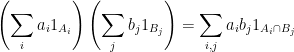
  . Using the identity
  , the property that is closed under multiplication is equivalent to being closed under pairwise intersections. That is, is a
  -system.
Theorem 4 (Monotone Class Theorem) Let be a -system on a set , and be a vector subspace of satisfying
-
 for all
  .
.
- .
- is closed under bounded increasing limits.
Then,  .
.
Even though it is weaker than, and a direct consequence of, theorem 1 above, this is one of the more common versions of the monotone class theorem used in practise. It is also rather easier to prove than the more general theorem 1 above. I include a direct proof theorem 4 below, and will use it to prove all other versions of the monotone class theorem stated in this post.
Fubini’s theorem allowing the orders of multiple integrals to be commuted is a consequence of the monotone class theorem. For -algebras and  on sets and
  respectively, the product -algebra
  on the product space
  is, by definition, the -algebra generated by products
  over
over  and
and  . I state Fubini’s theorem for finite measures, although it is straightforward to extend to -finite measures using monotone convergence.
Lemma 5 (Fubini) Let  and
and  be finite measure spaces. Then, for every bounded -measurable function
  ,
,
-
 is -measurable w.r.t.
  .
.
-
 is -measurable w.r.t.
  .
.
-
 .
.
Proof: Let be the space of bounded -measurable functions for which the conclusion of the lemma holds. By linearity of the integrals, is a vector space, and, by monotone convergence, is closed under taking limits of uniformly bounded increasing sequences of functions. Next, let be the collection of over and , which is a -system generating the -algebra . For any  , writing
  gives,

These are measurable and, integrating w.r.t. and respectively gives,

So,  . In particular,
  . Then, theorem 4 says that contains all bounded -measurable functions . ⬜
In the next version of the monotone class theorem, we relax the conditions on so that it is no longer required to be a vector space. This does, however, require us to enforce closure under both bounded increasing and bounded decreasing sequences. It also requires us to enforce that is a vector space and contains , in addition to being closed under multiplication. That is, is an algebra.
Theorem 6 (Monotone Class Theorem) Let be a subalgebra of and satisfy,
- .
- is closed under bounded increasing and bounded decreasing limits.
Then, .
As an example, once the integrals of continuous real-valued functions on a bounded interval ![{[a,b]}](https://s0.wp.com/latex.php?latex=%7B%5Ba%2Cb%5D%7D&bg=ffffff&fg=000000&s=0&c=20201002) have been constructed (by, e.g., limits of Riemann sums), the integrals of all bounded measurable functions are uniquely determined by the dominated convergence property.
have been constructed (by, e.g., limits of Riemann sums), the integrals of all bounded measurable functions are uniquely determined by the dominated convergence property.
The monotone class theorem as given in theorem 6 also has a version starting from a -system of subsets of , rather than a general algebra . Given a -system , the identity
shows that the linear span of indicator functions over is closed under multiplication. If  , then this means that the linear span is an algebra, so the following is a consequence of theorem 6.
Theorem 7 (Monotone Class Theorem) Let be a -system on a set , such that , and satisfy,
- the linear span of
 is contained in .
- is closed under bounded increasing and bounded decreasing limits.
Then, .
As an example, for an interval ![{I=[a,b]\subseteq{\mathbb R}}](https://s0.wp.com/latex.php?latex=%7BI%3D%5Ba%2Cb%5D%5Csubseteq%7B%5Cmathbb+R%7D%7D&bg=ffffff&fg=000000&s=0&c=20201002) , we can let consist of the closed subintervals of
, we can let consist of the closed subintervals of  . For any function
  of the form
![\displaystyle f=\sum_{i=1}^nc_i 1_{[a_i,b_i]}](https://s0.wp.com/latex.php?latex=%5Cdisplaystyle++f%3D%5Csum_%7Bi%3D1%7D%5Enc_i+1_%7B%5Ba_i%2Cb_i%5D%7D+&bg=ffffff&fg=000000&s=0&c=20201002)
for real numbers  and
and  in , the integral is

The monotone class theorem shows that dominated convergence uniquely determines the extension of the integral to all bounded measurable functions .
Proof of the Monotone Class Theorem
I will give proofs of the various alternative versions of the monotone class theorem stated in theorems 1, 4, 6 and 7 above. In all cases, we have a -algebra and want to show that contains . The method is to first show that contains for . Then, will contain all `simple’ functions, defined as linear combinations of such indicator functions. We then finish off by approximating arbitrary bounded measurable functions by increasing limits of simple functions.
The following method of approximating arbitrary nonnegative measurable functions as increasing limits of simple functions is standard.
Lemma 8 Let be a -algebra on a set , and  denote the linear span of
  . Then, for any -measurable function
  , there exists an increasing sequence
  with
with  .
.
Proof: For any finite subset  write
write  . Letting
  , write
For convenience, I am using  . For any
  , we see that
  if and only if
  , so
, so

It follows that  whenever
  . Hence, if we let
  be an increasing sequence of finite subsets of such that
  is dense in , and set
  , then
  increases to . For example, we can choose

⬜
Lemma 8 has the following immediate consequence.
Corollary 9 Let be a vector space such that is closed under bounded increasing limits. Let be a -algebra such that for all . Then,  .
.
Proof: As is a vector space, it contains the linear span,  , of the indicator functions over . For any nonnegative
  , lemma 8 gives a sequence
  increasing to . Hence,
  . Finally, for any , then
  and
and  are in and, by the vector space property,
  is also in . ⬜
The proof of the monotone class theorem as stated in theorem 4 is now a straightforward application of the -system lemma
Proof of Theorem 4: Let be the collection of sets such that . By assumption of the theorem,  . We show that is a d-system. First, as by assumption, then
  . Next, for any
  in then,

so,  . Finally, if
  is an increasing sequence in with limit
  , then
  is an increasing sequence in with limit . As is closed under bounded increasing limits, , so is a d-system as claimed.
The -system lemma now states that  . In particular, for all
  . Corollary 9 gives . ⬜
We move on to the proofs of the alternative versions of the monotone class theorem, all of which will follow from theorem 4. First, it is helpful to use a bit of notation: say that a set is a monotone class if it is closed under bounded increasing and bounded decreasing limits. The monotone class generated by an arbitrary is the smallest monotone class containing , and will be denoted by  .
.
Lemma 10 Let be a vector subspace of . Then, is a vector space.
Proof: Fixing  , let be the collection of
  such that
  . Note that, if
  is a bounded and increasing or decreasing sequence, then so is
  . Setting
  , we see that
  , so . This shows that is a monotone class. By the vector space property, and, hence,
  . This shows that for all and .
Next, for any  , let
, let  denote the collection of such that
  . If
. If  is a bounded increasing or decreasing sequence, then so is
  . Setting
  , we have
  . and, hence, is a monotone class. By the vector space property,
  for any
  and, therefore,
  . We have shown that, if is in , then for all . Hence,
  . This gives
  , so that for all and in . ⬜
Lemma 10 allows us to quickly establish theorem 7 as a consequence of theorem 4.
Proof of Theorem 7: Let be the linear span of over . As is a monotone class containing , we have  . Then, by lemma 10, is a vector space. As
  , theorem 4 gives

as required. ⬜
We turn to the proofs of theorems 1 and 6. Here, we are given  satisfying some conditions, and need to show that . The idea is to show that the indicator functions are in for all sets
  in a -system generating . Unlike in the case of theorems 4 and 7, we are not given this at the outset. Instead, there is a bit more work to be done. When is an algebra, the idea is roughly as follows, for any .
- By the algebra property,
 is in , for any real polynomial
  .
.
- The Stone–Weierstrass theorem states that every continuous function
 can be uniformly approximated by polynomials on bounded intervals, from which it follows that
  .
.
- For any closed
 , the indicator function
  is a decreasing limit of continuous functions, so
  is in .
Using this approach, we prove the following.
Lemma 11 Let be a subalgebra of , and let be the collection of such that there exists a decreasing sequence  with
with  . Then,
- is a -system.
-
 for all and closed .
-
 .
.
Proof: Suppose that and  are in . Then, there exists (nonnegative) decreasing sequences
  such that and
  . Therefore,
  is a decreasing sequence in
  with
with

So,  , showing that is a -system.
Next, fixing and closed , we show that . Choose a sequence of continuous functions  decreasing to
  . For example, if
  is nonempty, we can take

where  is the distance from to . If is empty then, trivially, we can take
  .
.
The next step is to replace the continuous functions  by polynomials. As , it satisfies
  for some nonnegative real
  . We apply the Stone–Weierstrass theorem to find a sequence of polynomials
  with
with  on
on ![{[-K,K]}](https://s0.wp.com/latex.php?latex=%7B%5B-K%2CK%5D%7D&bg=ffffff&fg=000000&s=0&c=20201002) . Then, on this interval,
. Then, on this interval,

So,  is a sequence of polynomials, decreasing on , to the limit . As is contained in the algebra , the composition
  is also in . As the image of is contained in , is decreasing with limit

Hence, as required.
Finally, by the above, for any and closed ,  . As the Borel -algebra is generated by closed sets, is
  -measurable, showing that . ⬜
Lemma 11 enables us to reduce theorems 1 and 6 to the simpler version of the monotone class theorem given by theorem 4, which has already been proven above. It is convenient to start by establishing the following result, which will imply theorems 1 and 6.
Lemma 12 Let , where is an algebra and is a vector space such that is closed under bounded increasing limits. Then, .
Proof: Let be the collection of such that there exists a sequence  decreasing to . As
  is a bounded increasing sequence in , its limit,
  is in , so . Lemma 11 states that is a -system so, by the last statement of lemma 11, and by theorem 4,

as required. ⬜
Theorem 1 is an immediate consequence of the lemma.
Proof of Theorem 1: As is a vector space containing and , it contains the linear span of  , which I denote as
  . As is an algebra, lemma 12 gives

as required. ⬜
Theorem 6 is also an immediate consequence.
Proof of Theorem 6: As is a monotone class, it contains . Lemma 10 says that is a vector space. Applying lemma 12 with in place of ,

as required. ⬜


Hi. I read your posts since many years ago and it has helped me to advance with my thesis regarding optimal stopping time problems for Markov processes. Now I’m looking for a reference of precisely the functional monotone class theorem (theorem 1, here), to include in my bibliography and as I cannot make reference to this excelent post, could you help me with some references?
Greestings!
Hi!
In lemma 11 there seems to be some typo or error (or maybe I am missing something obvious).
I can’t really see the argument for why we have a decreasing sequence of polynomials q_n.
It is shown that p_n – p_[n+1] is greater than something negative = -2^(-n-1) – 2^(-n)
Then this is said to be equal to 3.(2^(-n-1) – 2^(-n)). So a minus sign has disappeared and some symbol “3.” has been added.
I cannot figure out what this is supposed to mean. It does not seem to mean 3 as an integer number and 2^(-n-1) – 2^(-n) as the decimal part, since this is a positive number and our number -2^(-n-1) – 2^(-n) is negative.
Maybe this is some kind of notation that has been explained elsewhere? Or maybe it is some common notation I have completely missed?