Pathwise Regularity of Optional and Predictable Processes

As I have mentioned before in these notes, when working with processes in continuous time, it is important to select a good modification. Typically, this means that we work with processes which are left or right continuous. However, in general, it can be difficult to show that the paths of a process satisfy such pathwise regularity. In this post I show that for optional and predictable processes, the section theorems introduced in the previous post can be used to considerably simplify the situation. Although they are interesting results in their own right, the main application in these notes will be to optional and predictable projection. Once the projections are defined, the results from this post will imply that they preserve certain continuity properties of the process paths.

Suppose, for example, that we have a continuous-time process X which we want to show to be right-continuous. It is certainly necessary that, for any sequence of times ${t_n\in{\mathbb R}_+}$ decreasing to a limit ${t}$ , ${X_{t_n}}$ almost-surely tends to ${X_t}$ . However, even if we can prove this for every possible decreasing sequence ${t_n}$ , it does not follow that X is right-continuous. As a counterexample, if ${\tau\colon\Omega\rightarrow{\mathbb R}}$ is any continuously distributed random time, then the process ${X_t=1_{\{t\le \tau\}}}$ is not right-continuous. However, so long as the distribution of ${\tau}$ has no atoms, X is almost-surely continuous at each fixed time t. It is remarkable, then, that if we generalise to look at sequences of stopping times, then convergence in probability along decreasing sequences of stopping times is enough to guarantee everywhere right-continuity of the process. At least, it is enough so long as we restrict consideration to optional processes.

As usual, we work with respect to a complete filtered probability space ${(\Omega,\mathcal{F},\{\mathcal{F}_t\}_{t\ge0},{\mathbb P})}$ . Two processes are considered to be the same if they are equal up to evanescence, and any pathwise property is said to hold if it holds up to evanescence. That is, a process is right-continuous if and only is it is everywhere right-continuous on a set of probability 1. All processes will be taken to be real-valued, and a process is said to have left (or right) limits if its left (or right) limits exist everywhere, up to evanescence, and are finite.

Theorem 1 Let X be an optional process. Then,

X is right-continuous if and only if ${X_{\tau_n}\rightarrow X_\tau}$ in probability, for each uniformly bounded sequence ${\tau_n}$ of stopping times decreasing to a limit ${\tau}$ .
X has right limits if and only if ${X_{\tau_n}}$ converges in probability, for each uniformly bounded decreasing sequence ${\tau_n}$ of stopping times.
X has left limits if and only if ${X_{\tau_n}}$ converges in probability, for each uniformly bounded increasing sequence ${\tau_n}$ of stopping times.

The `only if’ parts of these statements is immediate, since convergence everywhere trivially implies convergence in probability. The importance of this theorem is in the `if’ directions. That is, it gives sufficient conditions to guarantee that the sample paths satisfy the respective regularity properties.

Note that conditions for left-continuity are absent from the statements of Theorem 1. In fact, left-continuity does not follow from the corresponding property along sequences of stopping times. Consider, for example, a Poisson process, X. This is right-continuous but not left-continuous. However, its jumps occur at totally inaccessible times. This implies that, for any sequence ${\tau_n}$ of stopping times increasing to a finite limit ${\tau}$ , it is true that ${X_{\tau_n}}$ converges almost surely to ${X_\tau}$ . In light of such examples, it is even more remarkable that right-continuity and the existence of left and right limits can be determined by just looking at convergence in probability along monotonic sequences of stopping times. Theorem 1 will be proven below, using the optional section theorem.

For predictable processes, we can restrict attention to predictable stopping times. In this case, we obtain a condition for left-continuity as well as for right-continuity.

Theorem 2 Let X be a predictable process. Then,

X is right-continuous if and only if ${X_{\tau_n}\rightarrow X_\tau}$ in probability, for each uniformly bounded sequence ${\tau_n}$ of predictable stopping times decreasing to a limit ${\tau}$ .
X is left-continuous if and only if ${X_{\tau_n}\rightarrow X_\tau}$ in probability, for each uniformly bounded sequence ${\tau_n}$ of predictable stopping times increasing to a limit ${\tau}$ .
X has right limits if and only if ${X_{\tau_n}}$ converges in probability, for each uniformly bounded decreasing sequence ${\tau_n}$ of predictable stopping times.
X has left limits if and only if ${X_{\tau_n}}$ converges in probability, for each uniformly bounded increasing sequence ${\tau_n}$ of predictable stopping times.

Again, the proof is given below, and relies on the predictable section theorem.

Theorems 1 and 2 can alternatively be stated in terms of convergence of expectations. So long as the processes satisfy sufficient integrability properties, then convergence of expectations is a significantly weaker condition than convergence in probability. For example, if X is a uniformly bounded process then, by bounded convergence, all of the limits along sequences of stopping times stated in the results above still hold after taking expectations. More generally, using convergence of expectations for uniformly integrable sequences, requiring X to be of class (DL) is sufficient for this to be true. In fact, at the cost of dropping the `only if’ directions of the statements, we only require the even milder property that X is integrable at the necessary random times.

Theorem 3 Let X be an optional process such that ${X_\tau}$ is integrable for each uniformly bounded stopping time ${\tau}$ . Then,

if ${X_\tau}$ is integrable and ${{\mathbb E}[X_{\tau_n}]\rightarrow{\mathbb E}[X_\tau]}$ for each uniformly bounded sequence ${\tau_n}$ of stopping times decreasing to a limit ${\tau}$ , then X is right-continuous.
if ${{\mathbb E}[X_{\tau_n}]}$ converges for each uniformly bounded decreasing sequence ${\tau_n}$ of stopping times, then X has right limits.
if ${{\mathbb E}[X_{\tau_n}]}$ converges for each uniformly bounded increasing sequence ${\tau_n}$ of stopping times, then X has left limits.

This is almost exactly the same as Theorem 1 other than the use of the weaker condition of convergence in expectation in place of convergence in probability. In a similar way, Theorem 2 can be restated using the weaker conditions of convergence in expectation.

Theorem 4 Let X be a predictable process such that ${X_\tau}$ is integrable for each uniformly bounded predictable stopping time ${\tau}$ . Then,

if ${X_\tau}$ is integrable and ${{\mathbb E}[X_{\tau_n}]\rightarrow{\mathbb E}[X_\tau]}$ for each uniformly bounded sequence ${\tau_n}$ of predictable stopping times decreasing to a limit ${\tau}$ , then X is right-continuous.
if ${{\mathbb E}[X_{\tau_n}]\rightarrow{\mathbb E}[X_\tau]}$ for each uniformly bounded sequence ${\tau_n}$ of predictable stopping times increasing to a limit ${\tau}$ , then X is left-continuous.
if ${{\mathbb E}[X_{\tau_n}]}$ converges for each uniformly bounded decreasing sequence ${\tau_n}$ of predictable stopping times, then X has right limits.
if ${{\mathbb E}[X_{\tau_n}]}$ converges for each uniformly bounded increasing sequence ${\tau_n}$ of predictable stopping times, then X has left limits.

The proofs of the above theorems will be given soon. Note that the first statements of each of these theorems involves the limits ${\tau}$ of decreasing sequences of stopping times. We did not restrict to the cases where ${\tau}$ is itself a stopping time, which would have given slightly stronger statements. In the usual situation, where the underlying filtration is right-continuous, this is automatic in any case. For Theorems 1 and 2 it is possible to restrict to the case where ${\tau}$ is a stopping time, but this is just a small strengthening of the statements so, for simplicity, I do not do this. Similarly, the second statements of Theorems 2 and 4 involve the limits of increasing sequences of predictable stopping times. However, increasing limits of predictable stopping times are predictable, regardless of whether or not the filtration satisfies the usual conditions. So, the restriction that ${\tau}$ is predictable could be stated if prefered, but it makes no real difference.

The underlying ideas behind the above theorems are provided in Chapter IV of the book Capacités et processes stochastiques (Springer-Verlag, 1972) by Claude Dellacherie. Actually, in this post, I am considering rather more than that stated in Dellacherie, although the ideas and method of proof will be similar. For one thing, Dellacherie restricts attention to uniformly bounded processes which removes any possible issues regarding integrability and ensures that all limits are finite. He also restricts attention to convergence in expectations, and does not state the versions involving convergence in probability given in Theorems 1 and 2 above, which somewhat reduces the number of statements to be proven. Furthermore, he restricts attention to the most important cases of left-continuity for predictable processes, and right-continuity and cadlag paths for optional processes. For reference, the result for left-continuity of predictable processes is given by Theorem T24 of Dellacherie and the result for right-continuity and cadlag paths of optional processes is in Theorem T28.

Between them, Theorems 1 to 4 consist of fourteen separate statements, all of which I will prove below. The large number of statements to be proven does mean that this post is rather long, but the underlying ideas are really the same for all of them. As noted above, the `only if’ direction of the statements of Theorems 1 and 2 is immediate anyway, so I do not explicitly consider these below. The proofs will be organised by separately considering each regularity property in turn — right-continuity, right limits, left-continuity and, finally, left limits.

Continuity at stopping times

The reduction of pathwise continuity to continuity along sequences of stopping times will be done in two stages. The first step is to reduce it to continuity at each stopping time, which is done by the following lemma. Note that, we do not actually require the process to be optional or predictable here. Progressive measurability is sufficient. As we are not assuming right-continuity of the filtration, we will instead look at stopping times with respect to the right limits, ${\{\mathcal{F}_{t+}\}_{t\ge0}}$ of the filtration.

Lemma 5 Let X be a progressively measurable process.

If, at each bounded ${\mathcal{F}_+}$ stopping time, X is almost surely right-continuous, then X is right-continuous everywhere (up to evanescence).
If, at each bounded ${\mathcal{F}_+}$ stopping time, X almost surely has right limits, then X has right limits everywhere (up to evanescence).
If, at each bounded predictable stopping time, X almost surely has left limits, then X has left limits everywhere (up to evanescence).

Proof: First, note that by replacing a stopping time ${\tau}$ by ${\tau\wedge T}$ for arbitrarily large real T, we can drop the constraint that the stopping times are bounded in the statements of the lemma. Instead, we require each respective condition to hold almost surely on the event ${\{\tau < \infty\}}$ .

I previously gave a proof that right-continuous adapted processes are optional, in the sense that they are measurable with respect to the sigma-algebra generated by sets ${[\tau,\infty)}$ for stopping times ${\tau}$ . There, it was shown that such processes can be uniformly approximated by processes which are explicitly right-continuous and generated by the required sigma-algebra. In fact, that proof only really required the weaker hypothesis that X is progressive and is almost surely right-continuous at each stopping time, which then implies the first statement of the lemma above. I now give a self-contained proof of the first statement of the lemma, although it is based on the method just mentioned.

For X to be right-continuous, we need to show that the process

$\displaystyle Z_t=\limsup_{s\downarrow t}\lvert X_s-X_t\rvert$

is evanescent. It is enough to show that ${Z\le\epsilon}$ (up to evanescence) for any given ${\epsilon > 0}$ .

Without loss of generality, assume that the underlying filtration is right-continuous. Let ${\mathcal{T}}$ be the set of stopping times ${\tau}$ such that ${1_{[0,\tau)}Z\le\epsilon}$ , up to evanescence. As ${\mathcal{T}}$ is closed under taking the supremum of countable sequences, it must contain its essential supremum ${\tau={\rm ess\;sup}\mathcal{T}}$ . To conclude that ${Z\le\epsilon}$ , it only needs to be shown that ${\tau=\infty}$ (almost surely). Consider

$\displaystyle \sigma = \inf\left\{t > \tau\colon \lvert X_t-X_\tau\rvert > \epsilon/2\right\}$

which, by the debut theorem is a stopping time. On the interval ${[\tau,\sigma)}$ , X is confined to the range ${[X_\tau-\epsilon/2,X_\tau+\epsilon/2]}$ , which has width ${\epsilon}$ . Hence, ${Z\le\epsilon}$ on this interval, showing that ${\sigma\in\mathcal{T}}$ . Whenever ${\tau < \infty}$ , the hypothesis of the first statement above says that X is right-continuous at ${\tau}$ and, hence, ${\sigma > \tau}$ . However, by definition of the essential supremum, ${\sigma\le\tau}$ (almost surely), showing that ${\tau=\infty}$ (a.s.) as required.

The second statement can be proved in a very similar way, replacing the process Z above by

$\displaystyle Z_t=\limsup_{u,v\downarrow\downarrow t}\lvert X_u-X_v\rvert.$

Again, we assume without loss of generality that the underlying filtration is right-continuous, and need to show that ${Z\le\epsilon}$ , up to evanescence, for any ${\epsilon > 0}$ . As above, let ${\mathcal{T}}$ be the set of stopping times ${\tau}$ for which ${1_{[0,\tau)}Z\le\epsilon}$ holds up to evanescence. The essential supremum ${\tau={\rm ess\;sup}\mathcal{T}}$ is itself in ${\mathcal{T}}$ . By the hypothesis of the second statement of the lemma, the limit ${X_{\tau+}=\lim_{t\downarrow\downarrow\tau}X_t}$ exists whenever ${\tau < \infty}$ . Define

$\displaystyle \sigma=\inf\left\{t > \tau\colon \lvert X_t - X_{\tau+}\rvert > \epsilon/2\right\}$

which, by the debut theorem, is a stopping time. On the interval ${(\tau, \sigma)}$ , X is confined to the range ${[X_{\tau+}-\epsilon/2,X_{\tau+}+\epsilon/2]}$ , which has width ${\epsilon}$ . Hence, ${Z\le\epsilon}$ on this interval, so ${\sigma\in\mathcal{T}}$ . Whenever ${\tau < \infty}$ , the definition of ${X_{\tau+}}$ implies that ${\sigma > \tau}$ . However, ${\sigma\le\tau}$ by the definition of the essential supremum, showing that ${\tau=\infty}$ (a.s.) as required.

For the final statement, define the processes

$\displaystyle \setlength\arraycolsep{2pt} \begin{array}{rl} \displaystyle X^+_{t-}&\displaystyle=\limsup_{s\uparrow\uparrow t}X_s,\smallskip\\ \displaystyle X^-_{t-}&\displaystyle=\liminf_{s\uparrow\uparrow t}X_s. \end{array}$

(1)

These are predictable processes taking values in the extended reals ${\bar{\mathbb R}={\mathbb R}\cup\{\pm\infty\}}$ . For X to have left limits, we need to show that ${X^-=X^+}$ is finite everywhere. From the third statement of the lemma, ${X^-_{\tau-}=X^+_{\tau-}\not=\pm\infty}$ (a.s.) at each finite predictable stopping time ${\tau}$ . So, by predictable section, ${X^-_{\cdot-}=X^+_{\cdot-}\not=\pm\infty}$ up to evanescence. ⬜

I did not include left-continuity in the lemma above. I now show that almost-sure left continuity at each predictable stopping time is sufficient although, as shown by the example of a Poisson process, it does require the hypothesis that X is predictable.

Lemma 6 Let X be a predictable process. If, at each bounded predictable stopping time, X is almost surely left-continuous, then X is left-continuous everywhere (up to evanescence).

Proof: Letting ${X^-_{t-}}$ and ${X^+_{t-}}$ be the predictable processes defined by (1), left-continuity at a finite predictable stopping time ${\tau}$ is equivalent to the equality ${X^-_{\tau-}=X^+_{\tau-}=X_\tau}$ . Then, predictable section implies that ${X^-_{\cdot-}=X^+_{\cdot-}=X_\cdot}$ up to evanescence, so X is left-continuous. ⬜

Right-Continuity

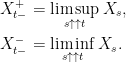
I now move on to proving sufficiency of the conditions in Theorems 1 to 4 for the respective pathwise properties to hold. Starting with right-continuity, define the right upper and lower limits of X at each time t,

$\displaystyle \setlength\arraycolsep{2pt} \begin{array}{rl} \displaystyle X^+_{t+}&\displaystyle=\limsup_{s\downarrow\downarrow t}X_s,\smallskip\\ \displaystyle X^-_{t+}&\displaystyle=\liminf_{s\downarrow\downarrow t}X_s. \end{array}$

(2)

We know that these are progressively measurable processes whenever X is progressive, so long as the underlying filtration is right-continuous. The following lemma will allow us to reduce the proof of right-continuity to an application of Lemma 5. Since the proofs for optional and predictable processes are almost identical, I deal with both cases simultaneously. This does entail a liberal use of the term `respectively‘ throughout these proofs, but avoids writing out near identical duplicate statements and proofs for the optional and predictable cases.

Lemma 7 Let X be an optional (respectively, predictable) process, ${a\in{\mathbb R}}$ , and ${\tau}$ be an ${\mathcal{F}_+}$ stopping time such that ${X^+_{\tau+} > a}$ whenever ${\tau < \infty}$ .

Then, there exists a sequence, ${\tau_n}$ , of stopping times (resp., predictable stopping times) decreasing to ${\tau}$ such that ${X_{\tau_n} > a}$ whenever ${\tau_n < \infty}$ .

Proof: For each n, consider the set

$\displaystyle S = (\tau,\tau+1/n]\cap\{X > a\}.$

Using the fact that the process ${1_{(\tau,\tau+1/n]}}$ is left-continuous and adapted, hence predictable, and that X is optional (resp., predictable), it follows that S is optional (resp., predictable). So, by the section theorem, there exists a (resp., predictable) stopping time ${\tau_n^0}$ with ${[\tau_n^0]\subseteq S}$ and

$\displaystyle {\mathbb P}\left(\tau_n^0 < \infty\right) > {\mathbb P}(\pi_\Omega(S))-2^{-n}.$

When ${\tau < \infty}$ , the condition that ${X^+_{\tau+} > a}$ implies that ${X > a}$ at some times in the interval ${(\tau,\tau+1/n]}$ . Hence, ${\{\tau < \infty\}\subseteq\pi_\Omega(S)}$ and,

$\displaystyle {\mathbb P}\left(\tau < \infty, \tau_n^0=\infty\right) ={\mathbb P}(\tau < \infty)-{\mathbb P}(\tau_n^0 < \infty) < 2^{-n}.$

(3)

The Borel-Cantelli lemma implies that, almost surely, ${\tau_n^0 < \infty}$ for large n whenever ${\tau < \infty}$ . By construction, ${X_{\tau_n^0} > a}$ and ${\tau < \tau_n^0\le\tau+1/n}$ whenever ${\tau^0_n < \infty}$ , so ${\tau_n^0\rightarrow\tau}$ almost surely.

Finally, setting

$\displaystyle \tau_n=\tau_1^0\wedge\tau_2^0\wedge\cdots\wedge\tau_n^0$

gives a sequence of (resp., predictable) stopping times almost surely decreasing to ${\tau}$ and with ${X_{\tau_n} > a}$ whenever ${\tau_n < \infty}$ . The `almost sure’ restriction can be removed, if preferred, by simply setting ${\tau_n=\tau}$ on the zero probability event that ${\tau_n}$ does not tend to ${\tau}$ . ⬜

Applying Lemmas 5 and 7, it is now relatively straightforward to give a proof of the first statements of Theorems 1 and 2. That is, continuity in probability computed along decreasing sequences of stopping times is sufficient to guarantee pathwise right-continuity.

Lemma 8 Let X be an optional (resp., predictable) process such that, for each uniformly bounded sequence of stopping times (resp., predictable stopping times) ${\tau_n}$ decreasing to a limit ${\tau}$ , ${X_{\tau_n}}$ tends to ${X_\tau}$ in probability. Then, X is right-continuous.

Proof: Letting ${\tau}$ be an ${\mathcal{F}_+}$ stopping time, by Lemma 5 it is enough to show that X is almost surely right-continuous at ${\tau}$ whenever ${\tau < \infty}$ . To do this, it is enough to show that ${X^+_{\tau+}\le X_{\tau}}$ (i.e., that it is right lower semicontinuous) as continuity follows by applying the same result to both ${X}$ and ${-X}$ . I use proof by contradiction so, suppose that ${X^+_{\tau+} > X_\tau}$ with positive probability. Then, by countable additivity, there must be an ${a\in{\mathbb Q}}$ such that

$\displaystyle X^+_{\tau+} > a > X_\tau.$

(4)

holds with positive probability. By setting ${\tau = \infty}$ on the event that (4) fails, we suppose that (4) holds whenever ${\tau}$ is finite.

Lemma 7 gives a sequence of (resp., predictable) stopping times ${\tau_n}$ decreasing to ${\tau}$ such that ${X_{\tau_n} > a}$ whenever ${\tau_n < \infty}$ . Now, fix a time ${T > 0}$ such that ${\tau < T}$ with positive probability. Then,

$\displaystyle \liminf_{n\rightarrow\infty} X_{\tau_n\wedge T}\ge a > X_{\tau\wedge T}$

whenever ${\tau < T}$ . So, ${X_{\tau_n\wedge T}}$ does not converge to ${X_{\tau\wedge T}}$ in probability, contradicting the hypothesis of the lemma. ⬜

Similarly, the proof of the first statements of Theorems 3 and 4 is now straightforward.

Lemma 9 Let X be an optional (resp., predictable) process such that ${X_\tau}$ is integrable for each ${\mathcal{F}_+}$ stopping time ${\tau}$ . Suppose that, for each uniformly bounded sequence of stopping times (resp., predictable stopping times) ${\tau_n}$ decreasing to a limit ${\tau}$ , ${{\mathbb E}[X_{\tau_n}]}$ tends to ${{\mathbb E}[X_\tau]}$ . Then, X is right-continuous.

Proof: Suppose that ${\tau_n\downarrow\tau}$ is as in the proof of Lemma 8. So, (4) holds whenever ${\tau < \infty}$ and ${X_{\tau_n} > a}$ when ${\tau_n < \infty}$ . Letting ${T}$ be a fixed time such that ${\tau < T}$ with positive probability,

$\displaystyle X_{\tau_n\wedge T}-X_{\tau\wedge T} > a - X_\tau > 0$

when ${\tau_n < T}$ . So,

$\displaystyle {\mathbb E}[X_{\tau_n\wedge T}-X_{\tau\wedge T}] \ge {\mathbb E}[1_{\{\tau_n < T\}}(a - X_\tau)] +{\mathbb E}[1_{\{\tau_n\ge T > \tau\}}(X_T-X_{\tau})].$

Taking the limit as n goes to infinity, and using dominated convergence,

$\displaystyle \liminf_{n\rightarrow\infty}{\mathbb E}[X_{\tau_n\wedge T}-X_{\tau\wedge T}] \ge {\mathbb E}[1_{\{\tau < T\}}(a-X_\tau)] > 0$

contradicting the hypothesis of the lemma. ⬜

Right Limits

I now move on to the proofs of existence of right limits, which follows along very similar lines as the proof above for right-continuity. The main difference here is that, the construction of a sequence of stopping times at which X lies above a level ${a}$ is replaced by a sequence on which X oscillates between two levels ${a}$ and ${b}$ . This will ensure that X does not converge to any limit along such a sequence of times, allowing a proof by contradiction similar to that used for Lemma 8 to be applied. So, the following result will play the same role in the argument here as Lemma 7 did for the proof of right-continuity above. The proof also follows in a very similar way to that given for Lemma 7.

Lemma 10 Let X be an optional (resp., predictable) process, ${a > b\in{\mathbb R}}$ , and ${\tau}$ be a ${\mathcal{F}_+}$ stopping time such that

$\displaystyle X^+_{\tau+} > a > b > X^-_{\tau+}$ (5)

whenever ${\tau < \infty}$ .

Then, there exists a sequence, ${\tau_n}$ , of stopping times (resp., predictable stopping times) decreasing to ${\tau}$ such that, whenever ${\tau_n < \infty}$ , ${X_{\tau_n} > a}$ for n even and ${X_{\tau_n} < b}$ for n odd.

Proof: Choose a sequence ${\tau_n^0}$ of (resp., predictable) stopping times with ${\tau_n^0 > \tau}$ when ${\tau < \infty}$ , as follows. First, set ${\tau_1^0=\infty}$ . Then for each ${n > 1}$ , supposing that ${\tau_{n-1}^0}$ has already been chosen, consider the set,

$\displaystyle S=\begin{cases} (\tau,(\tau+1/n)\wedge\tau_{n-1}^0]\cap\{X > a\},&n{\rm\ even},\\ (\tau,(\tau+1/n)\wedge\tau_{n-1}^0]\cap\{X < b\},&n{\rm\ odd}. \end{cases}$

Using the fact that ${1_{(\tau,(\tau+1/n)\wedge\tau_{n-1}^0]}}$ is left-continuous and adapted, hence predictable, and that X is optional (resp., predictable), we see that S is optional (resp., predictable). Therefore, by the section theorem, there exists a (resp., predictable) stopping time ${\tau_n^0}$ with ${[\tau_n^0]\subseteq S}$ and

$\displaystyle {\mathbb P}\left(\tau_n^0 < \infty\right) > {\mathbb P}(\pi_\Omega(S))-2^{-n}.$

By construction, whenever ${\tau_n^0 < \infty}$ , we have ${\tau_n^0 \le(\tau+1/n)\wedge\tau_{n-1}^0}$ , and ${X_{\tau_n^0} > a}$ or ${X_{\tau_n^0} < b}$ for, respectively, even and odd n. Also, when ${\tau < \infty}$ , the condition that ${X^+_{\tau+}> a > b > X^-_{\tau+}}$ implies that each of the inequalities ${X > a}$ and ${X < b}$ are satisfied at some times in the interval ${(\tau,(\tau+1/n)\wedge\tau_{n-1}^0]}$ . Hence, ${\{\tau < \infty\}\subseteq\pi_\Omega(S)}$ and, as in (3) above,

$\displaystyle {\mathbb P}\left(\tau < \infty, \tau_n^0=\infty\right) ={\mathbb P}(\tau < \infty)-{\mathbb P}(\tau_n^0 < \infty) < 2^{-n}.$

So, the Borel-Cantelli lemma implies that, almost surely, ${\tau_n^0 < \infty}$ for large n, whenever ${\tau < \infty}$ . After the last n for which ${\tau_n^0}$ is infinite, the sequence ${\tau_n^0}$ is then decreasing to ${\tau}$ .

The sequence of stopping times required by the lemma is given by

$\displaystyle \setlength\arraycolsep{2pt} \begin{array}{rl} \displaystyle \tau_n&\displaystyle=\sup\{\tau_n^0,\tau_{n+1}^0,\ldots\}\smallskip\\ &\displaystyle=\begin{cases} \infty,& \textrm{if }\tau_m^0=\infty\textrm{ for some }m\ge n,\\ \tau_n^0,& \textrm{otherwise}. \end{cases} \end{array}$

The class of stopping times is closed under taking suprema of countable sequences (and similarly for predictable stopping times), so ${\tau_n}$ satisfies the required properties. ⬜

We now prove the second statement of Theorem 1 and third statement of Theorem 2. That is, under the stated conditions, the paths of X have right limits everywhere. This is a consequence of Lemmas 5 and 10 above, and the proof follows in a similar way as for Lemma 8.

Lemma 11 Let X be an optional (resp., predictable) process such that, for each uniformly bounded decreasing sequence of stopping times (resp., predictable stopping times) ${\tau_n}$ , ${X_{\tau_n}}$ converges in probability. Then, X has right limits.

Proof: Letting ${\tau}$ be an ${\mathcal{F}_+}$ stopping time, by Lemma 5 it is enough to show that X almost surely has right limits at ${\tau}$ whenever ${\tau < \infty}$ . To do this, it is enough to show that ${X^+_{\tau+}= X^-_{\tau+}}$ are both almost surely finite. I use proof by contradiction so, suppose that this is not the case. Then, either ${X^+_{\tau+} > X^-_{\tau+}}$ or ${X^+_{\tau+}=X^-_{\tau+}=\pm\infty}$ with positive probability.

Consider the case where ${\tau < \infty}$ and ${X^+_{\tau+} > X^-_{\tau+}}$ with positive probability. Then, by countable additivity, there exists ${a > b\in{\mathbb Q}}$ such that ${\tau < \infty}$ and inequality (5) holds with positive probability. We can suppose that (5) holds whenever ${\tau < \infty}$ by setting ${\tau=\infty}$ whenever it fails. By Lemma 10, there exists a sequence ${\tau_n}$ of (resp., predictable) stopping times decreasing to ${\tau}$ such that ${X_{\tau_n} > a}$ (n even) and ${X_{\tau_n} < b}$ (n odd) whenever ${\tau_n < \infty}$ . Choose a fixed time ${T}$ such that ${\tau < T}$ with positive probability. Then,

$\displaystyle \liminf_{n\rightarrow\infty}\left(X_{\tau_{2n}\wedge T}-X_{\tau_{2n+1}\wedge T}\right)\ge a-b > 0$

whenever ${\tau < T}$ . So, ${X_{\tau_n}}$ does not converge in probability, contradicting the hypothesis of the lemma.

Now consider the case where ${\tau < \infty}$ and ${X^+_{\tau+}=X^-_{\tau+}=\infty}$ with positive probability. The sequence of predictable stopping times ${\tau_n=\tau+1/n}$ decreases to ${\tau}$ and ${X_{\tau_n}\rightarrow\infty}$ with positive probability. Hence, ${X_{\tau_n}}$ does not converge in probability, contradicting the hypothesis of the lemma.

The case where ${X^+_{\tau+}=X^-_{\tau+}=-\infty}$ follows as above with ${X}$ replaced by ${-X}$ . ⬜

The proof of the second statement of Theorem 3 and the third statement of Theorem 4 follow in a similar way.

Lemma 12 Let X be an optional (resp., predictable) process such that ${X_\tau}$ is integrable for each uniformly bounded stopping time (resp., predictable stopping time) ${\tau}$ . Suppose that, for each uniformly bounded decreasing sequence of stopping times (resp., predictable stopping times) ${\tau_n}$ , ${{\mathbb E}[X_{\tau_n}]}$ converges to a finite limit. Then, X has right limits.

Proof: Let ${\tau_n\downarrow\tau}$ be as in the proof of Lemma 11 for the case where inequality (5) holds when ${\tau < \infty}$ . Choose a fixed time ${T}$ such that ${\tau < T}$ with positive probability. Then,

$\displaystyle {\mathbb E}\left[X_{\tau_{2n}\wedge T} - X_{\tau_{2n+1}\wedge T}\right] \ge {\mathbb E}\left[1_{\{\tau_{2n} < T\}}(a-b)\right] + {\mathbb E}\left[1_{\{\tau_{2n+1} < T \le \tau_{2n}\}}(X_T-b)\right].$

Letting n go to infinity and using dominated convergence,

$\displaystyle \liminf_{n\rightarrow\infty}{\mathbb E}\left[X_{\tau_{2n}\wedge T} - X_{\tau_{2n+1}\wedge T}\right]\ge{\mathbb E}[1_{\{\tau < T\}}(a-b)] > 0,$

giving the required contradiction with the hypothesis of the lemma.

Again, as in the proof of Lemma 11, consider the case with ${X^+_{\tau+} = X^-_{\tau+}=\infty}$ when ${\tau < \infty}$ . By Lemma 7, there exists a sequence ${\tau_n}$ of (resp., predictable) stopping times decreasing to ${\tau}$ satisfying ${X_{\tau_n} > 0}$ whenever ${\tau_n < \infty}$ . Choose a fixed time ${T}$ such that ${\tau < T}$ with positive probability. Then,

$\displaystyle X_{\tau_n\wedge T}= 1_{\{\tau_n < T\}}X_{\tau_n} + 1_{\{\tau_n\ge T\}}X_T.$

Letting n go to infinity and using dominated convergence,

$\displaystyle \liminf_{n\rightarrow\infty}{\mathbb E}[X_{\tau_n\wedge T}]= \liminf_{n\rightarrow\infty}{\mathbb E}[1_{\{\tau_n < T\}}X_{\tau_n}]+{\mathbb E}[1_{\{\tau\ge T\}}X_T].$

The sequence of random variables ${1_{\{\tau_n < T\}}X_{\tau_n}}$ is nonnegative and tends to infinity. So, by Fatou’s lemma, ${{\mathbb E}[X_{\tau_n\wedge T}]}$ tends to infinity, contradicting the hypothesis of the lemma. ⬜

Left-Continuity

I now move on to left-continuity. The approach is very similar to that for right-continuity above. However, approximating stopping times from the left tends to be more difficult than from the right and, for this reason, ${\tau}$ will be required to be predictable, The following will play the same role for left-continuity as Lemma 7 did for right-continuity. The predictable processes ${X^+_{t-}\ge X^-_{t-}}$ are defined as the left upper and lower limits of X given by (1) above.

Lemma 13 Let X be an optional (resp., predictable) process, ${a\in{\mathbb R}}$ , and ${\tau > 0}$ be a predictable stopping time such that ${X^+_{\tau-} > a}$ whenever ${\tau < \infty}$ .

Then, there exists a sequence, ${\tau_n}$ , of stopping times (resp., predictable stopping times) increasing to ${\tau}$ such that ${X_{\tau_n} > a}$ whenever ${\tau_n < \infty}$ .

Proof: Let ${\sigma_n}$ be a sequence of stopping times announcing ${\tau}$ . For each ${n\ge1}$ consider the set

$\displaystyle S = (\sigma_n,\tau)\cap\{X > a\}.$

As ${1_{(\sigma_n,\tau)}}$ is the limit of the left-continuous adapted processes ${1_{(\sigma_n,\sigma_m]}}$ as m goes to infinity, it is predictable. Then, since X is optional (resp., predictable), S is also optional (resp., predictable). By the section theorem, there exists a (resp., predictable) stopping time ${\tau_n^0}$ with ${[\tau_n^0]\subseteq S}$ and

$\displaystyle {\mathbb P}\left(\tau_n^0 < \infty\right) > {\mathbb P}\left(\pi_\Omega(S)\right)-2^{-n}.$

By construction, ${\sigma_n < \tau_n^0 < \tau}$ and ${X_{\tau_n^0} > a}$ whenever ${\tau_n^0 < \infty}$ . As ${X^+_{\tau-} > a}$ , ${X > a}$ for some times in the interval ${(\sigma_n,\tau)}$ whenever ${\tau < \infty}$ . Hence, ${\{\tau < \infty\}\subseteq\pi_\Omega(S)}$ and, as in (3) above,

$\displaystyle {\mathbb P}\left(\tau < \infty, \tau_n^0 = \infty\right)\le{\mathbb P}\left(\pi_\Omega(S)\cap\{\tau_n^0=\infty\}\right) < 2^{-n}.$

By the Borel-Cantelli lemma, when ${\tau < \infty}$ then, almost surely, ${\tau_n^0 < \infty}$ for large n. So, ${\tau^0_n}$ tends to ${\tau}$ from the left. The sequence of stopping times required by the lemma is now given by

$\displaystyle \tau_n=\tau_n^0\wedge\tau_{n+1}^0\wedge\cdots.$

As ${\sigma_n < \tau_n\le\tau}$ , this sequence increases to ${\tau}$ . As the sequence ${\tau_n^0}$ (and any subsequence) tends to ${\tau}$ from the left, it must attain its minimum. So, for each n, we have ${\tau_n=\tau_m^0}$ for some m and, hence, ${X_{\tau_n} > a}$ whenever ${\tau_n < \infty}$ . Finally, for each fixed n, write ${\tau_n}$ as the limit of the sequence ${\tau_{nm} = \tau^0_n\wedge\cdots\wedge\tau^0_m}$ as m goes to infinity. As this is a sequence of (resp., predictable) stopping times and is eventually constant when ${\tau_n}$ is finite, it follows that ${\tau_n}$ is a stopping time (resp., a predictable stopping time). ⬜

Lemma 13 is now applied to prove the second statement of Theorem 2. The proof is analogous to the one for right-continuity given for Lemma 8 above. However, as we will apply Lemma 6, we only prove the result in the case of predictable X.

Lemma 14 Let X be a predictable process such that, for each uniformly bounded increasing sequence of predictable stopping times ${\tau_n\rightarrow\tau}$ , ${X_{\tau_n}}$ tends to ${X_\tau}$ in probability. Then, X is left-continuous.

Proof: Letting ${\tau > 0}$ be a finite predictable stopping time, by Lemma 6 it is enough to show that X is almost surely left-continuous at ${\tau}$ or, equivalently, ${X^-_{\tau-}=X^+_{\tau-}=X_\tau}$ . To do this, it is enough to show that ${X^+_{\tau-}\le X_{\tau}}$ , and then the inequality ${X^-_{\tau-}\ge X_\tau}$ will follow in the same way (or, by applying the same argument to ${-X}$ ). I use proof by contradiction so, suppose that ${X^+_{\tau-} > X_\tau}$ with positive probability. By countable additivity, there must be an ${a\in{\mathbb Q}}$ such that

$\displaystyle X^+_{\tau-} > a > X_\tau$

(6)

holds with positive probability. The event on which (6) holds is ${\mathcal{F}_{\tau-}}$ -measurable, so if we set ${\tau=\infty}$ on the event that it fails then ${\tau}$ will remain a predictable stopping time. So, we suppose that (6) holds whenever ${\tau}$ is finite.

Lemma 13 gives a sequence of predictable stopping times ${\tau_n}$ increasing to ${\tau}$ such that ${X_{\tau_n} > a}$ whenever ${\tau_n < \infty}$ . Then, choosing any fixed time T with ${{\mathbb P}(\tau\le T) > 0}$ ,

$\displaystyle \liminf_{n\rightarrow\infty}X_{\tau_n\wedge T}\ge a > X_{\tau\wedge T},$

whenever ${\tau\le T}$ . This contradicts the hypothesis that ${X_{\tau_n\wedge T}\rightarrow X_{\tau\wedge T}}$ in probability. ⬜

The proof of the second statement of Theorem 4 follows similarly, and is analogous to the one given for Lemma 9 above.

Lemma 15 Let X be a predictable process such that ${X_\tau}$ is integrable for each uniformly bounded predictable stopping time ${\tau}$ . Suppose that, for each uniformly bounded sequence of predictable stopping times ${\tau_n}$ increasing to a limit ${\tau}$ , ${{\mathbb E}[X_{\tau_n}]}$ tends to ${{\mathbb E}[X_\tau]}$ . Then, X is left-continuous.

Proof: As in the proof of Lemma 14, we just need to consider a predictable stopping time ${\tau}$ satisfying (6) whenever ${\tau < \infty}$ , and show that ${{\mathbb P}(\tau < \infty)=0}$ . By Lemma 13, there exists a sequence ${\tau_n}$ of predictable stopping times increasing to ${\tau}$ satisfying ${X_{\tau_n} > a}$ whenever ${\tau_n < \infty}$ .

Supposing that ${\tau < \infty}$ with positive probability, consider a fixed time T such that ${\tau\le T}$ with positive probability. Then,

$\displaystyle {\mathbb E}[X_{\tau_n\wedge T}-X_{\tau\wedge T}]\ge{\mathbb E}\left[1_{\{\tau_n \le T\}}(a-X_{\tau\wedge T})\right].$

Applying dominated convergence,

$\displaystyle \liminf_{n\rightarrow\infty}{\mathbb E}[X_{\tau_n\wedge T}-X_{\tau\wedge T}]\ge{\mathbb E}\left[1_{\{\tau \le T\}}(a-X_\tau)\right] > 0,$

giving the required contradiction. ⬜

Left Limits

I finally prove that the paths of X have left limits under the appropriate hypotheses. This extends the argument above for the case of left-continuity in a similar way to how we extended the argument above for right-continuity to prove the existence of right limits. Start with the following, which is analogous to Lemma 10 above.

Lemma 16 Let X be an optional (resp., predictable) process, ${a > b\in{\mathbb R}}$ , and ${\tau > 0}$ be a predictable stopping time satisfying

$\displaystyle X^+_{\tau-} > a > b > X^-_{\tau-}$ (7)

whenever ${\tau < \infty}$ .

Then, there exists a sequence, ${\tau_n}$ , of stopping times (resp., predictable stopping times) increasing to ${\tau}$ such that whenever ${\tau_n < \infty}$ , ${X_{\tau_n} > a}$ for n even and ${X_{\tau_n} < b}$ for n odd.

Proof: By Lemma 13, there exists sequences, ${\tau_n^+}$ and ${\tau_n^-}$ , of (resp., predictable) stopping times increasing to ${\tau}$ such that, ${X_{\tau_n^+} > a}$ whenever ${\tau_n^+ < \infty}$ and ${X_{\tau_n^-} < b}$ whenever ${\tau_n^- < \infty}$ .

Inductively define the sequence ${\tau_n}$ as follows. Set ${\tau_0=0}$ and, for each ${n > 0}$ , set

$\displaystyle \tau_n=\inf\left\{\tau^+_m\colon m\ge n, \tau^+_m > \tau_{n-1}\right\}$

for n even and,

$\displaystyle \tau_n=\inf\left\{\tau^-_m\colon m\ge n, \tau^-_m > \tau_{n-1}\right\}$

for n odd. By construction, ${\tau_n}$ is increasing to ${\tau}$ . Also, whenever ${\tau_n < \infty}$ and n is even, then ${\tau_n=\tau^+_m}$ for some m, so ${X_\tau > a}$ . Similarly, ${X_\tau < b}$ when ${\tau_n < \infty}$ and n is odd.

It only remains to be shown that ${\tau_n}$ are (resp., predictable) stopping times, which we do by induction. Assuming that ${\tau_{n-1}}$ is a stopping time, the event ${A_m=\{\tau_m^+ > \tau_{n-1}\}}$ is in ${\mathcal{F}_{\tau^+_m-}}$ for each m. This is seen by noting that ${1_{A_m}}$ is the value of the left-continuous and adapted process ${1_{(\tau_{n-1},\infty)}}$ at time ${\tau_m^+}$ . Then, let ${(\tau_m)_{A_m}}$ denote the time equal to ${\tau_m}$ on the event ${A_m}$ and ${\infty}$ otherwise. This is a stopping time (resp., is a predictable stopping time). Considering, without loss of generality, the case where n is even, then ${\tau_n}$ is the limit of the eventually constant sequence

$\displaystyle (\tau^+_n)_{A_n}\wedge(\tau^+_{n+1})_{A_{n+1}}\wedge\cdots\wedge(\tau^+_m)_{A_m}$

as m goes to infinity. Hence, ${\tau_n}$ is a stopping time (resp., is a predictable stopping time). ⬜

We apply Lemma 16 to prove the third statement of Theorem 1 and the fourth statement of Theorem 2.

Lemma 17 Let X be an optional (resp., predictable) process such that, for each uniformly bounded increasing sequence of stopping times (resp., predictable stopping times) ${\tau_n}$ , ${X_{\tau_n}}$ converges in probability. Then, X has left limits.

Proof: Letting ${\tau}$ be a finite predictable stopping time, by Lemma 5 it is enough to show that X almost surely has left limits at ${\tau}$ . To do this, it is enough to show that ${X^+_{\tau-}= X^-_{\tau-}}$ are both almost surely finite. I use proof by contradiction so, suppose that this is not the case. Then, either ${X^+_{\tau-} > X^-_{\tau-}}$ or ${X^+_{\tau-}=X^-_{\tau-}=\pm\infty}$ with positive probability.

Consider the case where ${X^+_{\tau-} > X^-_{\tau-}}$ with positive probability. By countable additivity, there exists ${a > b\in{\mathbb Q}}$ such that ${\tau < \infty}$ and inequality (7) holds with positive probability. We can suppose that (7) holds whenever ${\tau < \infty}$ by setting ${\tau=\infty}$ whenever it fails. Doing this preserves the property that ${\tau}$ is a predictable stopping time.

By Lemma 16, there exists a sequence ${\tau_n}$ of (predictable) stopping times increasing to ${\tau}$ such that ${X_{\tau_{2n}} > a}$ and ${X_{\tau_{2n+1}} < b}$ whenever these times are finite. Then, for any fixed time T with ${{\mathbb P}(\tau\le T) > 0}$ ,

$\displaystyle \liminf_{n\rightarrow\infty}\left(X_{\tau_{2n}\wedge T}-X_{\tau_{2n+1}\wedge T}\right)\ge 1_{\{\tau\le T\}}(a-b),$

which is positive with positive probability. So, ${X_{\tau_n}}$ does not converge in probability, contradicting the hypothesis of the lemma.

Now consider the case where ${X^+_{\tau-}=X^-_{\tau-}=\infty}$ with positive probability. Setting ${\tau=\infty}$ when this equality fails, we suppose that ${X^+_{\tau-}=X^-_{\tau-}=\infty}$ whenever ${\tau < \infty}$ . Lemma 13 gives a sequence, ${\tau_n}$ , of predictable stopping times increasing to ${\tau}$ such that ${X_{\tau_n} > 0}$ whenever ${\tau_n < \infty}$ (we do not actually require this property of ${X_{\tau_n}}$ here). Then, ${X_{\tau_n}\rightarrow\infty}$ with positive probability, contradicting the condition that ${X_{\tau_n}}$ converges in probability.

The case where ${X^+_{\tau-}=X^-_{\tau-}=-\infty}$ follows as above with ${X}$ replaced by ${-X}$ . ⬜

Finally, the proofs of the third statement of Theorem 3 and the fourth statement of Theorem 4 follow in a similar way.

Lemma 18 Let X be an optional (resp., predictable) process such that ${X_\tau}$ is integrable for each uniformly bounded stopping time (resp., predictable stopping time) ${\tau}$ . Suppose that, for each uniformly bounded increasing sequence of stopping times (resp., predictable stopping times) ${\tau_n}$ , ${{\mathbb E}[X_{\tau_n}]}$ converges to a finite limit. Then, X has left limits.

Proof: Let ${\tau_n\uparrow\tau}$ be as in the proof of Lemma 17 for the case where inequality (7) holds when ${\tau < \infty}$ . Then, choosing a fixed time T with ${{\mathbb P}(\tau\le T) > 0}$ ,

$\displaystyle X_{\tau_{2n}\wedge T} - X_{\tau_{2n+1}\wedge T} \ge 1_{\{\tau_{2n+1} \le T\}}(a-b) + 1_{\{\tau_{2n} \le T < \tau_{2n+1}\}}(a-X_T).$

Taking expectations and letting n go to infinity, using dominated convergence,

$\displaystyle \liminf_{n\rightarrow\infty}{\mathbb E}\left[X_{\tau_{2n}\wedge T} - X_{\tau_{2n+1}\wedge T}\right]\ge{\mathbb E}[1_{\{\tau\le T\}}(a-b)] > 0,$

giving the required contradiction with the hypothesis of the lemma.

Again, as in the proof of Lemma 17, consider the case with ${X^+_{\tau-} = X^-_{\tau-}=\infty}$ whenever ${\tau < \infty}$ and let ${\tau_n\uparrow\tau}$ be (resp., predictable) stopping times with ${X_{\tau_n} > 0}$ whenever ${\tau_n < \infty}$ . Let T be a fixed time with ${{\mathbb P}(\tau\le T) > 0}$ . The sequence ${X_{\tau_n\wedge T}}$ is bounded below by the integrable random variable ${X_T\wedge 0}$ and tends to ${\infty}$ on the event ${\{\tau\le T\}}$ so, by Fatou’s lemma,

$\displaystyle \liminf_{n\rightarrow\infty}{\mathbb E}\left[X_{\tau_n\wedge T}\right]=\infty$

contradicting the condition of the lemma. ⬜

Notes

Note that Theorems 1 and 2 are almost immediate consequences of Theorems 3 and 4. In the case where X is a uniformly bounded process then this is indeed the case. For example, suppose that X is optional and that ${X_{\tau_n}\rightarrow X_{\tau}}$ in probability for any bounded sequence ${\tau_n}$ of stopping times decreasing to a limit ${\tau}$ . Using bounded convergence, ${{\mathbb E}[X_{\tau_n}]}$ tends to ${{\mathbb E}[X_\tau]}$ , and the first statement of Theorem 3 implies that X is right-continuous. For bounded processes, this proves the first statement of Theorem 1 as a corollary of Theorem 3. This argument can be extended to unbounded processes by applying a continuous, bounded and strictly increasing function ${\varphi\colon{\mathbb R}\rightarrow{\mathbb R}}$ to X. For example, ${\varphi(x)=x/(1+\lvert x\rvert)}$ . If we set ${Y=\varphi(X)}$ and X satisfies the property that ${X_{\tau_n}\rightarrow X_\tau}$ for all bounded sequences ${\tau_n}$ of stopping times decreasing to a limit ${\tau}$ , then Y satisfies the same property. So, ${{\mathbb E}[Y_{\tau_n}]\rightarrow{\mathbb E}[Y_\tau]}$ and, assuming that X is optional, the first statement of Theorem 3 says that Y is right-continuous. Then, ${X=\varphi^{-1}(Y)}$ is also right-continuous. So, the first statement of Theorem 1 does indeed follow immediately from the corresponding statement of Theorem 3. Precisely the same argument applies for each of the statements of Theorems 1 and 2 which involving left and right continuity. So, it is not strictly necessary to provide proofs of these. For the statements involving left and right limits, however, it is not quite so straightforward. Even if we show that Y has right limits, for example, it does not follow that X has right limits. It could be the case that the right limits of Y are outside of the range of ${\varphi}$ . Then, the right limits of ${\varphi^{-1}(Y)}$ can go to plus or minus infinity, and it can only be concluded that X has right limits in the extended reals. I did not use such ideas above, and instead gave proofs of all statements, as it worked out easier to prove the statements of Theorems 1 and 2 first and then extend the arguments to Theorems 3 and 4 and, in any case, the idea mentioned does not simplify things much.

One thought on “Pathwise Regularity of Optional and Predictable Processes”

Stat Prof says:

2 March 24 at 8:29 PM

Hi, I’ve been enjoying your blog and have learned a lot through reading it — though the modest depth of my measure theory training holds me back at times. The reliance of the theory on left- or right-continuous processes seems extremely prevalent across much of the literature. I have a question on which you may be able to shed some light, as I have interest in the properties of a stochastic process that is neither. Suppose you have a pair of random variables (X,D), where X > 0 may have a distribution with both discrete and continuous components and D is 0-1 binary. Assume these are defined on a complete filtered probability space, where the right-continuous filtration ${\cal F}_t$ is generated by the processes $I(X\leq t, D = 1), I(X\leq t, D = 0)$ for $t >= 0.$ Define the process of interest as $Y(t) = I(X \geq t) - I(X = t) D.$ This process has paths that are neither left-continuous nor right-continuous. It is adapted since it can be written in terms of the processes above. But is it progressively measurable? I ask because you can rewrite the process as $Y(t) = (1-D) I(X \geq t) + D I(X > t)$ — this is a sum of 2 processes, each being progressively measurable, but one is left-continuous and the other is right continuous. Let $\tau$ be the first time at which $Y(t) = 0$ . Is $\tau$ a ${\cal F}_t$ -stopping time? Thanks!

	Anonymous on About
	Anonymous on About
	Anonymous on The Stochastic Integral
	Anonymous on Bessel Processes
	Anonymous on Bessel Processes
	Stat Prof on Pathwise Regularity of Optiona…
	Yang Chu on Spitzer’s Formula
	Anonymous on About
	Anonymous on Continuous Processes with Inde…
	Anonymous on Continuous Processes with Inde…

Pathwise Regularity of Optional and Predictable Processes

Continuity at stopping times

Right-Continuity

Right Limits

Left-Continuity

Left Limits

Notes

Published by George Lowther

One thought on “Pathwise Regularity of Optional and Predictable Processes”

Leave a comment Cancel reply

Continuity at stopping times

Right-Continuity

Right Limits

Left-Continuity

Left Limits

Notes

Related

Published by George Lowther

One thought on “Pathwise Regularity of Optional and Predictable Processes”

Leave a comment Cancel reply