Proof of Optional and Predictable Section

In this post I give a proof of the theorems of optional and predictable section. These are often considered among the more advanced results in stochastic calculus, and many texts on the subject skip their proofs entirely. The approach here makes use of the measurable section theorem but, other than that, is relatively self-contained and will not require any knowledge of advanced topics beyond basic properties of probability measures.

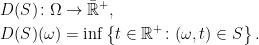
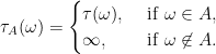
Given a probability space ${(\Omega,\mathcal F,{\mathbb P})}$ we denote the projection map from ${\Omega\times{\mathbb R}^+}$ to ${\Omega}$ by

$\displaystyle \setlength\arraycolsep{2pt} \begin{array}{rl} &\displaystyle\pi_\Omega\colon \Omega\times{\mathbb R}^+\rightarrow\Omega,\smallskip\\ &\displaystyle\pi_\Omega(\omega,t)=\omega. \end{array}$

For a set ${S\subseteq\Omega\times{\mathbb R}^+}$ then, by construction, for every ${\omega\in\pi_\Omega(S)}$ there exists a ${t\in{\mathbb R}^+}$ with ${(\omega,t)\in S}$ . Measurable section states that this choice can be made in a measurable way. That is, assuming that the probability space is complete, ${\pi_\Omega(S)}$ is measurable and there is a measurable section ${\tau\colon\Omega\rightarrow{\mathbb R}^+}$ satisfying ${\tau\in S}$ . I use the shorthand ${\tau\in S}$ to mean ${(\omega,\tau(\omega))\in S}$ , and it is convenient to extend the domain of ${\tau}$ to all of ${\Omega}$ by setting ${\tau=\infty}$ outside of ${\pi_\Omega(S)}$ . So, we consider random times taking values in the extended nonnegative real numbers ${\bar{\mathbb R}^+={\mathbb R}^+\cup\{\infty\}}$ . The property that ${\tau\in S}$ whenever ${\tau < \infty}$ can be expressed by stating that the graph of ${\tau}$ is contained in S, where the graph is defined as

$\displaystyle [\tau]\equiv\left\{(\omega,t)\in\Omega\times{\mathbb R}^+\colon t=\tau(\omega)\right\}.$

The optional section theorem is a significant extension of measurable section which is very important to the general theory of stochastic processes. It starts with the concept of stopping times and with the optional sigma-algebra on ${\Omega\times{\mathbb R}^+}$ . Then, it says that if S is optional its section ${\tau}$ can be chosen to be a stopping time. However, there is a slight restriction. It might not be possible to define such ${\tau}$ everywhere on ${\pi_\Omega(S)}$ , but instead only up to a set of positive probability ${\epsilon}$ , where ${\epsilon}$ can be made as small as we like. There is also a corresponding predictable section theorem, which says that if S is in the predictable sigma-algebra, its section ${\tau}$ can be chosen to be a predictable stopping time.

I give precise statements and proofs of optional and predictable section further below, and also prove a much more general section theorem which applies to any collection of random times satisfying a small number of required properties. Optional and predictable section will follow as consequences of this generalised section theorem.

Both the optional and predictable sigma-algebras, as well as the sigma-algebra used in the generalised section theorem, can be generated by collections of stochastic intervals. Any pair of random times ${\sigma,\tau\colon\Omega\rightarrow\bar{\mathbb R}^+}$ defines a stochastic interval,

$\displaystyle [\sigma,\tau)\equiv\left\{(\omega,t)\in\Omega\times{\mathbb R}^+\colon\sigma(\omega)\le t < \tau(\omega)\right\}.$

The debut of a set ${S\subseteq\Omega\times{\mathbb R}^+}$ is defined to be the random time

$\displaystyle \setlength\arraycolsep{2pt} \begin{array}{rl} &\displaystyle D(S)\colon\Omega\rightarrow\bar{\mathbb R}^+,\smallskip\\ &\displaystyle D(S)(\omega)=\inf\left\{t\in{\mathbb R}^+\colon(\omega,t)\in S\right\}. \end{array}$

In general, even if S is measurable, its debut need not be, although it can be shown to be measurable in the case that the probability space is complete. For a random time ${\tau}$ and a measurable set ${A\subseteq\Omega}$ , we use ${\tau_A}$ to denote the restriction of ${\tau}$ to A defined by

$\displaystyle \tau_A(\omega)=\begin{cases} \tau(\omega),&{\rm\ if\ }\omega\in A,\\ \infty,&{\rm\ if\ }\omega\not\in A. \end{cases}$

We start with the general situation of a collection of random times ${\mathcal T}$ satisfying a few required properties and show that, for sufficiently simple subsets of ${\Omega\times{\mathbb R}^+}$ , the section can be chosen to be almost surely equal to the debut. It is straightforward that the collection of all stopping times defined with respect to some filtration do indeed satisfy the required properties for ${\mathcal T}$ , but I also give a proof of this further below. A nonempty collection ${\mathcal A}$ of subsets of a set X is called an algebra, Boolean algebra or, alternatively, a ring, if it is closed under finite unions, finite intersections, and under taking the complement ${A^c=X\setminus A}$ of sets ${A\in\mathcal A}$ . Recall, also, that ${\mathcal A_\delta}$ represents the countable intersections of A, which is the collection of sets of the form ${\bigcap_nA_n}$ for sequences ${A_1,A_2,\ldots}$ in ${\mathcal A}$ .

Lemma 1 Let ${(\Omega,\mathcal F,{\mathbb P})}$ be a probability space and ${\mathcal T}$ be a collection of measurable times ${\tau\colon\Omega\rightarrow\bar{\mathbb R}^+}$ satisfying,

the constant function ${\tau=0}$ is in ${\mathcal T}$ .

${\sigma\wedge\tau}$ and ${\sigma_{\{\sigma < \tau\}}}$ are in ${\mathcal T}$ , for all ${\sigma,\tau\in\mathcal T}$ .

${\sup_n\mathcal\tau_n\in\mathcal T}$ for all sequences ${\tau_1,\tau_2,\cdots}$ in ${\mathcal T}$ .

Then, letting ${\mathcal A}$ be the collection of finite unions of stochastic intervals ${[\sigma,\tau)}$ over ${\sigma,\tau\in\mathcal T}$ , we have the following,

${\mathcal A}$ is an algebra on ${\Omega\times{\mathbb R}^+}$ .

for all ${S\in\mathcal A_\delta}$ , its debut satisfies
$\displaystyle [D(S)]\subseteq S,\ \{D(S) < \infty\}=\pi_\Omega(S),$

and there is a ${\tau\in\mathcal T}$ with ${[\tau]\subseteq[D(S)]}$ and ${\tau = D(S)}$ almost surely.

Continue reading “Proof of Optional and Predictable Section” →

The Projection Theorems

In this post, I introduce the concept of optional and predictable projections of jointly measurable processes. Optional projections of right-continuous processes and predictable projections of left-continuous processes were constructed in earlier posts, with the respective continuity conditions used to define the projection. These are, however, just special cases of the general theory. For arbitrary measurable processes, the projections cannot be expected to satisfy any such pathwise regularity conditions. Instead, we use the measurability criteria that the projections should be, respectively, optional and predictable.

The projection theorems are a relatively straightforward consequence of optional and predictable section. However, due to the difficulty of proving the section theorems, optional and predictable projection is generally considered to be an advanced or hard part of stochastic calculus. Here, I will make use of the section theorems as stated in an earlier post, but leave the proof of those until after developing the theory of projection.

As usual, we work with respect to a complete filtered probability space ${(\Omega,\mathcal{F},\{\mathcal{F}\}_{t\ge0},{\mathbb P})}$ , and only consider real-valued processes. Any two processes are considered to be the same if they are equal up to evanescence. The optional projection is then defined (up to evanescence) by the following.

Theorem 1 (Optional Projection) Let X be a measurable process such that ${{\mathbb E}[1_{\{\tau < \infty\}}\lvert X_\tau\rvert\;\vert\mathcal{F}_\tau]}$ is almost surely finite for each stopping time ${\tau}$ . Then, there exists a unique optional process ${{}^{\rm o}\!X}$ , referred to as the optional projection of X, satisfying

$\displaystyle 1_{\{\tau < \infty\}}{}^{\rm o}\!X_\tau={\mathbb E}[1_{\{\tau < \infty\}}X_\tau\,\vert\mathcal{F}_\tau]$ (1)

almost surely, for each stopping time ${\tau}$ .

Predictable projection is defined similarly.

Theorem 2 (Predictable Projection) Let X be a measurable process such that ${{\mathbb E}[1_{\{\tau < \infty\}}\lvert X_\tau\rvert\;\vert\mathcal{F}_{\tau-}]}$ is almost surely finite for each predictable stopping time ${\tau}$ . Then, there exists a unique predictable process ${{}^{\rm p}\!X}$ , referred to as the predictable projection of X, satisfying

$\displaystyle 1_{\{\tau < \infty\}}{}^{\rm p}\!X_\tau={\mathbb E}[1_{\{\tau < \infty\}}X_\tau\,\vert\mathcal{F}_{\tau-}]$ (2)

almost surely, for each predictable stopping time ${\tau}$ .

Continue reading “The Projection Theorems” →

Pathwise Regularity of Optional and Predictable Processes

As I have mentioned before in these notes, when working with processes in continuous time, it is important to select a good modification. Typically, this means that we work with processes which are left or right continuous. However, in general, it can be difficult to show that the paths of a process satisfy such pathwise regularity. In this post I show that for optional and predictable processes, the section theorems introduced in the previous post can be used to considerably simplify the situation. Although they are interesting results in their own right, the main application in these notes will be to optional and predictable projection. Once the projections are defined, the results from this post will imply that they preserve certain continuity properties of the process paths.

Suppose, for example, that we have a continuous-time process X which we want to show to be right-continuous. It is certainly necessary that, for any sequence of times ${t_n\in{\mathbb R}_+}$ decreasing to a limit ${t}$ , ${X_{t_n}}$ almost-surely tends to ${X_t}$ . However, even if we can prove this for every possible decreasing sequence ${t_n}$ , it does not follow that X is right-continuous. As a counterexample, if ${\tau\colon\Omega\rightarrow{\mathbb R}}$ is any continuously distributed random time, then the process ${X_t=1_{\{t\le \tau\}}}$ is not right-continuous. However, so long as the distribution of ${\tau}$ has no atoms, X is almost-surely continuous at each fixed time t. It is remarkable, then, that if we generalise to look at sequences of stopping times, then convergence in probability along decreasing sequences of stopping times is enough to guarantee everywhere right-continuity of the process. At least, it is enough so long as we restrict consideration to optional processes.

As usual, we work with respect to a complete filtered probability space ${(\Omega,\mathcal{F},\{\mathcal{F}_t\}_{t\ge0},{\mathbb P})}$ . Two processes are considered to be the same if they are equal up to evanescence, and any pathwise property is said to hold if it holds up to evanescence. That is, a process is right-continuous if and only is it is everywhere right-continuous on a set of probability 1. All processes will be taken to be real-valued, and a process is said to have left (or right) limits if its left (or right) limits exist everywhere, up to evanescence, and are finite.

Theorem 1 Let X be an optional process. Then,

X is right-continuous if and only if ${X_{\tau_n}\rightarrow X_\tau}$ in probability, for each uniformly bounded sequence ${\tau_n}$ of stopping times decreasing to a limit ${\tau}$ .

X has right limits if and only if ${X_{\tau_n}}$ converges in probability, for each uniformly bounded decreasing sequence ${\tau_n}$ of stopping times.

X has left limits if and only if ${X_{\tau_n}}$ converges in probability, for each uniformly bounded increasing sequence ${\tau_n}$ of stopping times.

The `only if’ parts of these statements is immediate, since convergence everywhere trivially implies convergence in probability. The importance of this theorem is in the `if’ directions. That is, it gives sufficient conditions to guarantee that the sample paths satisfy the respective regularity properties.

Note that conditions for left-continuity are absent from the statements of Theorem 1. In fact, left-continuity does not follow from the corresponding property along sequences of stopping times. Consider, for example, a Poisson process, X. This is right-continuous but not left-continuous. However, its jumps occur at totally inaccessible times. This implies that, for any sequence ${\tau_n}$ of stopping times increasing to a finite limit ${\tau}$ , it is true that ${X_{\tau_n}}$ converges almost surely to ${X_\tau}$ . In light of such examples, it is even more remarkable that right-continuity and the existence of left and right limits can be determined by just looking at convergence in probability along monotonic sequences of stopping times. Theorem 1 will be proven below, using the optional section theorem.

For predictable processes, we can restrict attention to predictable stopping times. In this case, we obtain a condition for left-continuity as well as for right-continuity.

Theorem 2 Let X be a predictable process. Then,

X is right-continuous if and only if ${X_{\tau_n}\rightarrow X_\tau}$ in probability, for each uniformly bounded sequence ${\tau_n}$ of predictable stopping times decreasing to a limit ${\tau}$ .

X is left-continuous if and only if ${X_{\tau_n}\rightarrow X_\tau}$ in probability, for each uniformly bounded sequence ${\tau_n}$ of predictable stopping times increasing to a limit ${\tau}$ .

X has right limits if and only if ${X_{\tau_n}}$ converges in probability, for each uniformly bounded decreasing sequence ${\tau_n}$ of predictable stopping times.

X has left limits if and only if ${X_{\tau_n}}$ converges in probability, for each uniformly bounded increasing sequence ${\tau_n}$ of predictable stopping times.

Again, the proof is given below, and relies on the predictable section theorem. Continue reading “Pathwise Regularity of Optional and Predictable Processes” →

The Section Theorems

Consider a probability space ${(\Omega,\mathcal{F},{\mathbb P})}$ and a subset S of ${{\mathbb R}_+\times\Omega}$ . The projection ${\pi_\Omega(S)}$ is the set of ${\omega\in\Omega}$ such that there exists a ${t\in{\mathbb R}_+}$ with ${(t,\omega)\in S}$ . We can ask whether there exists a map

$\displaystyle \tau\colon\pi_\Omega(S)\rightarrow{\mathbb R}_+$

such that ${(\tau(\omega),\omega)\in S}$ . From the definition of the projection, values of ${\tau(\omega)}$ satisfying this exist for each individual ${\omega}$ . By invoking the axiom of choice, then, we see that functions ${\tau}$ with the required property do exist. However, to be of use for probability theory, it is important that ${\tau}$ should be measurable. Whether or not there are measurable functions with the required properties is a much more difficult problem, and is answered affirmatively by the measurable selection theorem. For the question to have any hope of having a positive answer, we require S to be measurable, so that it lies in the product sigma-algebra ${\mathcal{B}({\mathbb R}_+)\otimes\mathcal{F}}$ , with ${\mathcal{B}({\mathbb R}_+)}$ denoting the Borel sigma-algebra on ${{\mathbb R}_+}$ . Also, less obviously, the underlying probability space should be complete. Throughout this post, ${(\Omega,\mathcal{F},{\mathbb P})}$ will be assumed to be a complete probability space.

It is convenient to extend ${\tau}$ to the whole of ${\Omega}$ by setting ${\tau(\omega)=\infty}$ for ${\omega}$ outside of ${\pi_\Omega(S)}$ . Then, ${\tau}$ is a map to the extended nonnegative reals ${\bar{\mathbb R}_+={\mathbb R}_+\cup\{\infty\}}$ for which ${\tau(\omega) < \infty}$ precisely when ${\omega}$ is in ${\pi_\Omega(S)}$ . Next, the graph of ${\tau}$ , denoted by ${[\tau]}$ , is defined to be the set of ${(t,\omega)\in{\mathbb R}_+\times\Omega}$ with ${t=\tau(\omega)}$ . The property that ${(\tau(\omega),\omega)\in S}$ whenever ${\tau(\omega) < \infty}$ is expressed succinctly by the inclusion ${[\tau]\subseteq S}$ . With this notation, the measurable selection theorem is as follows.

Theorem 1 (Measurable Selection) For any ${S\in\mathcal{B}({\mathbb R}_+)\otimes\mathcal{F}}$ , there exists a measurable ${\tau\colon\Omega\rightarrow\bar{\mathbb R}_+}$ such that ${[\tau]\subseteq S}$ and

$\displaystyle \left\{\tau < \infty\right\}=\pi_\Omega(S).$ (1)

As noted above, if it wasn’t for the measurability requirement then this theorem would just be a simple application of the axiom of choice. Requiring ${\tau}$ to be measurable, on the other hand, makes the theorem much more difficult to prove. For instance, it would not hold if the underlying probability space was not required to be complete. Note also that, stated as above, measurable selection implies that the projection of S is equal to a measurable set ${\{\tau < \infty\}}$ , so the measurable projection theorem is an immediate corollary. I will leave the proof of Theorem 1 for a later post, together with the proofs of the section theorems stated below.

A closely related problem is the following. Given a measurable space ${(X,\mathcal{E})}$ and a measurable function, ${f\colon X\rightarrow\Omega}$ , does there exist a measurable right-inverse on the image of ${f}$ ? This is asking for a measurable function, ${g}$ , from ${f(X)}$ to ${X}$ such that ${f(g(\omega))=\omega}$ . In the case where ${(X,\mathcal{E})}$ is the Borel space ${({\mathbb R}_+,\mathcal{B}({\mathbb R}_+))}$ , Theorem 1 says that it does exist. If S is the graph ${\{(t,f(t))\colon t\in{\mathbb R}_+\}}$ then ${\tau}$ will be the required right-inverse. In fact, as all uncountable Polish spaces are Borel-isomorphic to each other and, hence, to ${{\mathbb R}_+}$ , this result applies whenever ${(X,\mathcal{E})}$ is a Polish space together with its Borel sigma-algebra. Continue reading “The Section Theorems” →

Predictable Processes

In contrast to optional processes, the class of predictable processes was used extensively in the development of stochastic integration in these notes. They appeared as integrands in stochastic integrals then, later on, as compensators and in the Doob-Meyer decomposition. Since they are also central to the theory of predictable section and projection, I will revisit the basic properties of predictable processes now. In particular, any of the collections of sets and processes in the following theorem can equivalently be used to define the predictable sigma-algebra. As usual, we work with respect to a complete filtered probability space ${(\Omega,\mathcal{F},\{\mathcal{F}_t\}_{t\in{\mathbb R}_+},{\mathbb P})}$ . However, completeness is not actually required for the following result. All processes are assumed to be real valued, or take values in the extended reals ${\bar{\mathbb R}={\mathbb R}\cup\{\pm\infty\}}$ .

Theorem 1 The following collections of sets and processes each generate the same sigma-algebra on ${{\mathbb R}_+\times\Omega}$ .

{ ${[\tau,\infty)}$ : ${\tau}$ is a predictable stopping time}.

${Z1_{[\tau,\infty)}}$ as ${\tau}$ ranges over the predictable stopping times and Z over the ${\mathcal{F}_{\tau-}}$ -measurable random variables.

${\{A\times(t,\infty)\colon t\in{\mathbb R}_+,A\in\mathcal{F}_t\}\cup\{A\times\{0\}\colon A\in\mathcal{F}_0\}}$ .

The elementary predictable processes.

{ ${(\tau,\infty)}$ : ${\tau}$ is a stopping time} ${\cup}$ { ${A\times\{0\}\colon A\in\mathcal{F}_0}$ }.

The left-continuous adapted processes.

The continuous adapted processes.

Compare this with the analogous result for sets/processes generating the optional sigma-algebra given in the previous post. The proof of Theorem 1 is given further below. First, recall that the predictable sigma-algebra was previously defined to be generated by the left-continuous adapted processes. However, it can equivalently be defined by any of the collections stated in Theorem 1. To make this clear, I now restate the definition making use if this equivalence.

Definition 2 The predictable sigma-algebra, ${\mathcal{P}}$ , is the sigma-algebra on ${{\mathbb R}_+\times\Omega}$ generated by any of the collections of sets/processes in Theorem 1.

A stochastic process is predictable iff it is ${\mathcal{P}}$ -measurable.

Continue reading “Predictable Processes” →

Optional Processes

The optional sigma-algebra, ${\mathcal{O}}$ , was defined earlier in these notes as the sigma-algebra generated by the adapted and right-continuous processes. Then, a stochastic process is optional if it is ${\mathcal{O}}$ -measurable. However, beyond the definition, very little use was made of this concept. While right-continuous adapted processes are optional by construction, and were used throughout the development of stochastic calculus, there was no need to make use of the general definition. On the other hand, optional processes are central to the theory of optional section and projection. So, I will now look at such processes in more detail, starting with the following alternative, but equivalent, ways of defining the optional sigma-algebra. Throughout this post we work with respect to a complete filtered probability space ${(\Omega,\mathcal{F},\{\mathcal{F}_t\}_{t\in{\mathbb R}_+},{\mathbb P})}$ , and all stochastic processes will be assumed to be either real-valued or to take values in the extended reals ${\bar{\mathbb R}={\mathbb R}\cup\{\pm\infty\}}$ .

Theorem 1 The following collections of sets and processes each generate the same sigma-algebra on ${{\mathbb R}_+\times\Omega}$ .

{ ${[\tau,\infty)}$ : ${\tau}$ is a stopping time}.

${Z1_{[\tau,\infty)}}$ as ${\tau}$ ranges over the stopping times and Z over the ${\mathcal{F}_\tau}$ -measurable random variables.

The cadlag adapted processes.

The right-continuous adapted processes.

The optional-sigma algebra was previously defined to be generated by the right-continuous adapted processes. However, any of the four collections of sets and processes stated in Theorem 1 can equivalently be used, and the definitions given in the literature do vary. So, I will restate the definition making use of this equivalence.

Definition 2 The optional sigma-algebra, ${\mathcal{O}}$ , is the sigma-algebra on ${{\mathbb R}_+\times\Omega}$ generated by any of the collections of sets/processes in Theorem 1.

A stochastic process is optional iff it is ${\mathcal{O}}$ -measurable.

Continue reading “Optional Processes” →

Measurable Projection and the Debut Theorem

I will discuss some of the immediate consequences of the following deceptively simple looking result.

Theorem 1 (Measurable Projection) If ${(\Omega,\mathcal{F},{\mathbb P})}$ is a complete probability space and ${A\in\mathcal{B}({\mathbb R})\otimes\mathcal{F}}$ then ${\pi_\Omega(A)\in\mathcal{F}}$ .

The notation ${\pi_B}$ is used to denote the projection from the cartesian product ${A\times B}$ of sets A and B onto B. That is, ${\pi_B((a,b)) = b}$ . As is standard, ${\mathcal{B}({\mathbb R})}$ is the Borel sigma-algebra on the reals, and ${\mathcal{A}\otimes\mathcal{B}}$ denotes the product of sigma-algebras.

Theorem 1 seems almost obvious. Projection is a very simple map and we may well expect the projection of, say, a Borel subset of ${{\mathbb R}^2}$ onto ${{\mathbb R}}$ to be Borel. In order to formalise this, we could start by noting that sets of the form ${A\times B}$ for Borel A and B have an easily described, and measurable, projection, and the Borel sigma-algebra is the closure of the collection such sets under countable unions and under intersections of decreasing sequences of sets. Furthermore, the projection operator commutes with taking the union of sequences of sets. Unfortunately, this method of proof falls down when looking at the limit of decreasing sequences of sets, which does not commute with projection. For example, the decreasing sequence of sets ${S_n=(0,1/n)\times{\mathbb R}\subseteq{\mathbb R}^2}$ all project onto the whole of ${{\mathbb R}}$ , but their limit is empty and has empty projection.

There is an interesting history behind Theorem 1, as mentioned by Gerald Edgar on MathOverflow (1) in answer to The most interesting mathematics mistake? In a 1905 paper, Henri Lebesgue asserted that the projection of a Borel subset of the plane onto the line is again a Borel set (Lebesgue, (3), pp 191–192). This was based on the erroneous assumption that projection commutes with the limit of a decreasing sequence of sets. The mistake was spotted, in 1916, by Mikhail Suslin, and led to his investigation of analytic sets and to begin the study of what is now known as descriptive set theory. See Kanamori, (2), for more details. In fact, as was shown by Suslin, projections of Borel sets need not be Borel. So, by considering the case where ${\Omega={\mathbb R}}$ and ${\mathcal{F}=\mathcal{B}({\mathbb R})}$ , Theorem 1 is false if the completeness assumption is dropped. I will give a proof of Theorem 1 but, as it is a bit involved, this is left for a later post.

For now, I will state some consequences of the measurable projection theorem which are important to the theory of continuous-time stochastic processes, starting with the following. Throughout this post, the underlying probability space ${(\Omega,\mathcal{F})}$ is assumed to be complete, and stochastic processes are taken to be real-valued, or take values in the extended reals ${\bar{\mathbb R}={\mathbb R}\cup\{\pm\infty\}}$ , with time index ranging over ${{\mathbb R}_+}$ . For a first application of measurable projection, it allows us to show that the supremum of a jointly measurable processes is measurable.

Lemma 2 If X is a jointly measurable process and ${S\in\mathcal{B}(\mathbb{R}_+)}$ then ${\sup_{s\in S}X_s}$ is measurable.

Proof: Setting ${U=\sup_{s\in S}X_s}$ then, for each real K, ${U > K}$ if and only if ${X_s > K}$ for some ${s\in S}$ . Hence,

$\displaystyle U^{-1}\left((K,\infty]\right)=\pi_\Omega\left((S\times\Omega)\cap X^{-1}\left((K,\infty]\right)\right).$

By the measurable projection theorem, this is in ${\mathcal{F}}$ and, as sets of the form ${(K,\infty]}$ generate the Borel sigma-algebra on ${\mathbb{\bar R}}$ , U is ${\mathcal{F}}$ -measurable. ⬜

Next, the running maximum of a jointly measurable process is again jointly measurable.

Lemma 3 If X is a jointly measurable process then ${X^*_t\equiv\sup_{s\le t}X_s}$ is also jointly measurable.

Continue reading “Measurable Projection and the Debut Theorem” →

Optional Projection For Right-Continuous Processes

In filtering theory, we have a filtered probability space ${(\Omega,\mathcal{F},\{\mathcal{F}_t\}_{t\ge 0},{\mathbb P})}$ and a signal process ${\{X_t\}_{t\in{\mathbb R}_+}}$ . The sigma-algebra ${\mathcal{F}_t}$ represents the collection of events which are observable up to and including time t. The process X is not assumed to be adapted, so need not be directly observable. For example, we may only be able to measure an observation process ${Z_t=X_t+\epsilon_t}$ , which incorporates some noise ${\epsilon_t}$ , and generates the filtration ${\mathcal{F}_t}$ , so is adapted. The problem, then, is to compute an estimate for ${X_t}$ based on the observable data at time t. Looking at the expected value of X conditional on the observable data, we obtain the following estimate for X at each time ${t\in{\mathbb R}_+}$ ,

$\displaystyle Y_t={\mathbb E}[X_t\;\vert\mathcal{F}_t]{\rm\ \ (a.s.)}$

(1)

The process Y is adapted. However, as (1) only defines Y up to a zero probability set, it does not give us the paths of Y, which requires specifying its values simultaneously at the uncountable set of times in ${{\mathbb R}_+}$ . Consequently, (1) does not tell us the distribution of Y at random times. So, it is necessary to specify a good version for Y.

Optional projection gives a uniquely defined process which satisfies (1), not just at every time t in ${{\mathbb R}_+}$ , but also at all stopping times. The full theory of optional projection for jointly measurable processes requires the optional section theorem. As I will demonstrate, in the case where X is right-continuous, optional projection can be done by more elementary methods.

Throughout this post, it will be assumed that the underlying filtered probability space satisfies the usual conditions, meaning that it is complete and right-continuous, ${\mathcal{F}_{t+}=\mathcal{F}_t}$ . Stochastic processes are considered to be defined up to evanescence. That is, two processes are considered to be the same if they are equal up to evanescence. In order to apply (1), some integrability requirements need to imposed on X. Often, to avoid such issues, optional projection is defined for uniformly bounded processes. For a bit more generality, I will relax this requirement a bit and use prelocal integrability. Recall that, in these notes, a process X is prelocally integrable if there exists a sequence of stopping times ${\tau_n}$ increasing to infinity and such that

$\displaystyle 1_{\{\tau_n > 0\}}\sup_{t < \tau_n}\lvert X_t\rvert$

(2)

is integrable. This is a strong enough condition for the conditional expectation (1) to exist, not just at each fixed time, but also whenever t is a stopping time. The main result of this post can now be stated.

Theorem 1 (Optional Projection) Let X be a right-continuous and prelocally integrable process. Then, there exists a unique right-continuous process Y satisfying (1).

Uniqueness is immediate, as (1) determines Y, almost-surely, at each fixed time, and this is enough to uniquely determine right-continuous processes up to evanescence. Existence of Y is the important part of the statement, and the proof will be left until further down in this post.

The process defined by Theorem 1 is called the optional projection of X, and is denoted by ${{}^{\rm o}\!X}$ . That is, ${{}^{\rm o}\!X}$ is the unique right-continuous process satisfying

$\displaystyle {}^{\rm o}\!X_t={\mathbb E}[X_t\;\vert\mathcal{F}_t]{\rm\ \ (a.s.)}$

(3)

for all times t. In practise, the process X will usually not just be right-continuous, but will also have left limits everywhere. That is, it is cadlag.

Theorem 2 Let X be a cadlag and prelocally integrable process. Then, its optional projection is cadlag.

A simple example of optional projection is where ${X_t}$ is constant in t and equal to an integrable random variable U. Then, ${{}^{\rm o}\!X_t}$ is the cadlag version of the martingale ${{\mathbb E}[U\;\vert\mathcal{F}_t]}$ . Continue reading “Optional Projection For Right-Continuous Processes” →

Compensators of Counting Processes

A counting process, X, is defined to be an adapted stochastic process starting from zero which is piecewise constant and right-continuous with jumps of size 1. That is, letting ${\tau_n}$ be the first time at which ${X_t=n}$ , then

$\displaystyle X_t=\sum_{n=1}^\infty 1_{\{\tau_n\le t\}}.$

By the debut theorem, ${\tau_n}$ are stopping times. So, X is an increasing integer valued process counting the arrivals of the stopping times ${\tau_n}$ . A basic example of a counting process is the Poisson process, for which ${X_t-X_s}$ has a Poisson distribution independently of ${\mathcal{F}_s}$ , for all times ${t > s}$ , and for which the gaps ${\tau_n-\tau_{n-1}}$ between the stopping times are independent exponentially distributed random variables. As we will see, although Poisson processes are just one specific example, every quasi-left-continuous counting process can actually be reduced to the case of a Poisson process by a time change. As always, we work with respect to a complete filtered probability space ${(\Omega,\mathcal{F},\{\mathcal{F}_t\}_{t\ge0},{\mathbb P})}$ .

Note that, as a counting process X has jumps bounded by 1, it is locally integrable and, hence, the compensator A of X exists. This is the unique right-continuous predictable and increasing process with ${A_0=0}$ such that ${X-A}$ is a local martingale. For example, if X is a Poisson process of rate ${\lambda}$ , then the compensated Poisson process ${X_t-\lambda t}$ is a martingale. So, the compensator of X is the continuous process ${A_t=\lambda t}$ . More generally, X is said to be quasi-left-continuous if ${{\mathbb P}(\Delta X_\tau=0)=1}$ for all predictable stopping times ${\tau}$ , which is equivalent to the compensator of X being almost surely continuous. Another simple example of a counting process is ${X=1_{[\tau,\infty)}}$ for a stopping time ${\tau > 0}$ , in which case the compensator of X is just the same thing as the compensator of ${\tau}$ .

As I will show in this post, compensators of quasi-left-continuous counting processes have many parallels with the quadratic variation of continuous local martingales. For example, Lévy’s characterization states that a local martingale X starting from zero is standard Brownian motion if and only if its quadratic variation is ${[X]_t=t}$ . Similarly, as we show below, a counting process is a homogeneous Poisson process of rate ${\lambda}$ if and only if its compensator is ${A_t=\lambda t}$ . It was also shown previously in these notes that a continuous local martingale X has a finite limit ${X_\infty=\lim_{t\rightarrow\infty}X_t}$ if and only if ${[X]_\infty}$ is finite. Similarly, a counting process X has finite value ${X_\infty}$ at infinity if and only if the same is true of its compensator. Another property of a continuous local martingale X is that it is constant over all intervals on which its quadratic variation is constant. Similarly, a counting process X is constant over any interval on which its compensator is constant. Finally, it is known that every continuous local martingale is simply a continuous time change of standard Brownian motion. In the main result of this post (Theorem 5), we show that a similar statement holds for counting processes. That is, every quasi-left-continuous counting process is a continuous time change of a Poisson process of rate 1. Continue reading “Compensators of Counting Processes” →

Compensators of Stopping Times

The previous post introduced the concept of the compensator of a process, which is known to exist for all locally integrable semimartingales. In this post, I’ll just look at the very special case of compensators of processes consisting of a single jump of unit size.

Definition 1 Let ${\tau}$ be a stopping time. The compensator of ${\tau}$ is defined to be the compensator of ${1_{[\tau,\infty)}}$ .

So, the compensator A of ${\tau}$ is the unique predictable FV process such that ${A_0=0}$ and ${1_{[\tau,\infty)}-A}$ is a local martingale. Compensators of stopping times are sufficiently special that we can give an accurate description of how they behave. For example, if ${\tau}$ is predictable, then its compensator is just ${1_{\{\tau > 0\}}1_{[\tau,\infty)}}$ . If, on the other hand, ${\tau}$ is totally inaccessible and almost surely finite then, as we will see below, its compensator, A, continuously increases to a value ${A_\infty}$ which has the exponential distribution.

However, compensators of stopping times are sufficiently general to be able to describe the compensator of any cadlag adapted process X with locally integrable variation. We can break X down into a continuous part plus a sum over its jumps,

$\displaystyle X_t=X_0+X^c_t+\sum_{n=1}^\infty\Delta X_{\tau_n}1_{[\tau_n,\infty)}.$

(1)

Here, ${\tau_n > 0}$ are disjoint stopping times such that the union ${\bigcup_n[\tau_n]}$ of their graphs contains all the jump times of X. That they are disjoint just means that ${\tau_m\not=\tau_n}$ whenever ${\tau_n < \infty}$ , for any ${m\not=n}$ . As was shown in an earlier post, not only is such a sequence ${\tau_n}$ of the stopping times guaranteed to exist, but each of the times can be chosen to be either predictable or totally inaccessible. As the first term, ${X^c_t}$ , on the right hand side of (1) is a continuous FV process, it is by definition equal to its own compensator. So, the compensator of X is equal to ${X^c}$ plus the sum of the compensators of ${\Delta X_{\tau_n}1_{[\tau_n,\infty)}}$ . The reduces compensators of locally integrable FV processes to those of processes consisting of a single jump at either a predictable or a totally inaccessible time. Continue reading “Compensators of Stopping Times” →

	Anonymous on About
	Anonymous on About
	Anonymous on The Stochastic Integral
	Anonymous on Bessel Processes
	Anonymous on Bessel Processes
	Stat Prof on Pathwise Regularity of Optiona…
	Yang Chu on Spitzer’s Formula
	Anonymous on About
	Anonymous on Continuous Processes with Inde…
	Anonymous on Continuous Processes with Inde…