Proof of Optional and Predictable Section

In this post I give a proof of the theorems of optional and predictable section. These are often considered among the more advanced results in stochastic calculus, and many texts on the subject skip their proofs entirely. The approach here makes use of the measurable section theorem but, other than that, is relatively self-contained and will not require any knowledge of advanced topics beyond basic properties of probability measures.

Given a probability space ${(\Omega,\mathcal F,{\mathbb P})}$ we denote the projection map from ${\Omega\times{\mathbb R}^+}$ to ${\Omega}$ by

$\displaystyle \setlength\arraycolsep{2pt} \begin{array}{rl} &\displaystyle\pi_\Omega\colon \Omega\times{\mathbb R}^+\rightarrow\Omega,\smallskip\\ &\displaystyle\pi_\Omega(\omega,t)=\omega. \end{array}$

For a set ${S\subseteq\Omega\times{\mathbb R}^+}$ then, by construction, for every ${\omega\in\pi_\Omega(S)}$ there exists a ${t\in{\mathbb R}^+}$ with ${(\omega,t)\in S}$ . Measurable section states that this choice can be made in a measurable way. That is, assuming that the probability space is complete, ${\pi_\Omega(S)}$ is measurable and there is a measurable section ${\tau\colon\Omega\rightarrow{\mathbb R}^+}$ satisfying ${\tau\in S}$ . I use the shorthand ${\tau\in S}$ to mean ${(\omega,\tau(\omega))\in S}$ , and it is convenient to extend the domain of ${\tau}$ to all of ${\Omega}$ by setting ${\tau=\infty}$ outside of ${\pi_\Omega(S)}$ . So, we consider random times taking values in the extended nonnegative real numbers ${\bar{\mathbb R}^+={\mathbb R}^+\cup\{\infty\}}$ . The property that ${\tau\in S}$ whenever ${\tau < \infty}$ can be expressed by stating that the graph of ${\tau}$ is contained in S, where the graph is defined as

$\displaystyle [\tau]\equiv\left\{(\omega,t)\in\Omega\times{\mathbb R}^+\colon t=\tau(\omega)\right\}.$

The optional section theorem is a significant extension of measurable section which is very important to the general theory of stochastic processes. It starts with the concept of stopping times and with the optional sigma-algebra on ${\Omega\times{\mathbb R}^+}$ . Then, it says that if S is optional its section ${\tau}$ can be chosen to be a stopping time. However, there is a slight restriction. It might not be possible to define such ${\tau}$ everywhere on ${\pi_\Omega(S)}$ , but instead only up to a set of positive probability ${\epsilon}$ , where ${\epsilon}$ can be made as small as we like. There is also a corresponding predictable section theorem, which says that if S is in the predictable sigma-algebra, its section ${\tau}$ can be chosen to be a predictable stopping time.

I give precise statements and proofs of optional and predictable section further below, and also prove a much more general section theorem which applies to any collection of random times satisfying a small number of required properties. Optional and predictable section will follow as consequences of this generalised section theorem.

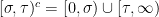
Both the optional and predictable sigma-algebras, as well as the sigma-algebra used in the generalised section theorem, can be generated by collections of stochastic intervals. Any pair of random times ${\sigma,\tau\colon\Omega\rightarrow\bar{\mathbb R}^+}$ defines a stochastic interval,

$\displaystyle [\sigma,\tau)\equiv\left\{(\omega,t)\in\Omega\times{\mathbb R}^+\colon\sigma(\omega)\le t < \tau(\omega)\right\}.$

The debut of a set ${S\subseteq\Omega\times{\mathbb R}^+}$ is defined to be the random time

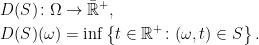
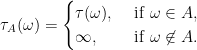
$\displaystyle \setlength\arraycolsep{2pt} \begin{array}{rl} &\displaystyle D(S)\colon\Omega\rightarrow\bar{\mathbb R}^+,\smallskip\\ &\displaystyle D(S)(\omega)=\inf\left\{t\in{\mathbb R}^+\colon(\omega,t)\in S\right\}. \end{array}$

In general, even if S is measurable, its debut need not be, although it can be shown to be measurable in the case that the probability space is complete. For a random time ${\tau}$ and a measurable set ${A\subseteq\Omega}$ , we use ${\tau_A}$ to denote the restriction of ${\tau}$ to A defined by

$\displaystyle \tau_A(\omega)=\begin{cases} \tau(\omega),&{\rm\ if\ }\omega\in A,\\ \infty,&{\rm\ if\ }\omega\not\in A. \end{cases}$

We start with the general situation of a collection of random times ${\mathcal T}$ satisfying a few required properties and show that, for sufficiently simple subsets of ${\Omega\times{\mathbb R}^+}$ , the section can be chosen to be almost surely equal to the debut. It is straightforward that the collection of all stopping times defined with respect to some filtration do indeed satisfy the required properties for ${\mathcal T}$ , but I also give a proof of this further below. A nonempty collection ${\mathcal A}$ of subsets of a set X is called an algebra, Boolean algebra or, alternatively, a ring, if it is closed under finite unions, finite intersections, and under taking the complement ${A^c=X\setminus A}$ of sets ${A\in\mathcal A}$ . Recall, also, that ${\mathcal A_\delta}$ represents the countable intersections of A, which is the collection of sets of the form ${\bigcap_nA_n}$ for sequences ${A_1,A_2,\ldots}$ in ${\mathcal A}$ .

Lemma 1 Let ${(\Omega,\mathcal F,{\mathbb P})}$ be a probability space and ${\mathcal T}$ be a collection of measurable times ${\tau\colon\Omega\rightarrow\bar{\mathbb R}^+}$ satisfying,

the constant function ${\tau=0}$ is in ${\mathcal T}$ .
${\sigma\wedge\tau}$ and ${\sigma_{\{\sigma < \tau\}}}$ are in ${\mathcal T}$ , for all ${\sigma,\tau\in\mathcal T}$ .
${\sup_n\mathcal\tau_n\in\mathcal T}$ for all sequences ${\tau_1,\tau_2,\cdots}$ in ${\mathcal T}$ .

Then, letting ${\mathcal A}$ be the collection of finite unions of stochastic intervals ${[\sigma,\tau)}$ over ${\sigma,\tau\in\mathcal T}$ , we have the following,

${\mathcal A}$ is an algebra on ${\Omega\times{\mathbb R}^+}$ .
for all ${S\in\mathcal A_\delta}$ , its debut satisfies
$\displaystyle [D(S)]\subseteq S,\ \{D(S) < \infty\}=\pi_\Omega(S),$

and there is a ${\tau\in\mathcal T}$ with ${[\tau]\subseteq[D(S)]}$ and ${\tau = D(S)}$ almost surely.

Proof: By construction, the collection ${\mathcal A}$ is closed under finite unions. Furthermore, the intersection of two stochastic intervals in ${\mathcal A}$

$\displaystyle [\sigma_1,\tau_1)\cap[\sigma_2,\tau_2)=[\sigma_1\vee\sigma_2,\tau_1\wedge\tau_2)$

is itself a stochastic interval, so ${\mathcal A}$ is closed under finite intersections. Noting that for any ${\tau}$ in ${\mathcal T}$ , ${\tau_{\{\tau < \tau\}}}$ is the constant function equal to infinity which, therefore, is in ${\mathcal T}$ , we see that the complement of a stochastic interval

$\displaystyle [\sigma,\tau)^c=[0,\sigma)\cup[\tau,\infty)$

is in ${\mathcal A}$ . So ${\mathcal A}$ is closed under set complements, and is an algebra.

The property ${\{D(S) < \infty\}=\pi_\Omega(S)}$ is immediate from the definition of the debut and holds for any ${S\subseteq\Omega\times{\mathbb R}^+}$ , using the fact that the infimum of a subset of ${{\mathbb R}^+}$ is finite if and only if the set is nonempty. Similarly, for ${S\in\mathcal A_\delta}$ , the fact that ${[D(S)]\subseteq S}$ does not require any of the properties of ${\mathcal T}$ . The slices,

$\displaystyle S_n(\omega)=\left\{t\in{\mathbb R}^+\colon (\omega,t)\in S\right\}$

are, by construction, finite unions of left-closed intervals. Hence, 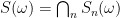${S(\omega)=\bigcap_nS_n(\omega)}$ is left-closed and, as any nonempty left-closed set contains its infimum, we have that ${[D(S)]}$ is contained in S.

We now show that the debut of a set ${S\in\mathcal A_\delta}$ is almost surely equal to a time in ${\mathcal T}$ . Let ${\mathcal S}$ be the set of all ${\tau\in\mathcal T}$ with ${\tau\le D(S)}$ , and ${\sigma}$ be the essential supremum of ${\mathcal S}$ . By standard properties of the essential supremum, we can write ${\sigma=\sup_n\sigma_n}$ for a sequence ${\sigma_n}$ in ${\mathcal S}$ . It follows that ${\sigma\in\mathcal T}$ and ${\sigma\le D(S)}$ , so ${\sigma}$ is in ${\mathcal S}$ . We will show that ${\sigma=D(S)}$ almost surely.

Write ${S=\bigcap_nS_n}$ for a sequence ${S_n\in\mathcal E}$ . Choosing any n, the time

$\displaystyle \tau_n=D([\sigma,\infty)\cap S_n)$

satisfies ${[\tau_n]\subseteq S_n}$ . As ${[\sigma,\infty)\cap S_n}$ is in ${\mathcal A}$ and can be expressed as a finite union ${\bigcup_{k=1}^m[\sigma_k,\tau_k)}$ ,

$\displaystyle \tau_n=\min_{1\le k\le m}D([\sigma_k,\tau_k))=\min_{1\le k\le m}(\sigma_k)_{\{\sigma_k < \tau_k\}}$

is in ${\mathcal T}$ . Using ${S_n\supseteq S}$ , it is immediate that ${\sigma\le\tau_n\le D(S)}$ . Hence, ${\tau\equiv\sup_n\tau_n}$ is in ${\mathcal S}$ . So, by the definition of the essential supremum, ${\tau\le\sigma}$ almost surely, in which case ${\tau=\sigma}$ . Furthermore, whenever ${\tau=\sigma}$ we necessarily have ${\tau_n=\sigma}$ for all n and, in this case, ${[\sigma]\subseteq\bigcap_nS_n=S}$ , so ${\sigma=D(S)}$ .

We have constructed ${\sigma\le\tau}$ in ${\mathcal T}$ such that ${\sigma=\tau}$ almost surely, and ${\sigma=D(S)}$ whenever ${\sigma=\tau}$ . It follows that the time ${\upsilon=\sigma_{\{\sigma\ge\tau\}}}$ is almost surely equal to ${D(S)}$ and ${[\upsilon]\subseteq[D(S)]}$ . To complete the proof, all that remains is to show that ${\upsilon}$ is in ${\mathcal T}$ . However, this follows from writing ${\upsilon=\sigma_{\{\sigma < \sigma_{\{\sigma < \tau\}}\}}}$ . ⬜

In order to apply lemma 1 to more general measurable sets S, it will be necessary to approximate by sets in ${\mathcal A_\delta}$ . This is done using the following standard lemma.

Lemma 2 Let ${(X,\mathcal E,\mu)}$ be a finite measure space and ${\mathcal A\subseteq\mathcal E}$ be an algebra generating ${\mathcal E}$ as a sigma-algebra. Then, for any ${A\in\mathcal E}$ and ${\epsilon > 0}$ , there exists a ${B\subseteq A}$ in ${\mathcal A_\delta}$ satisfying

$\displaystyle \mu(B) > \mu(A)-\epsilon.$ (1)

Proof: This is a standard application of the monotone class theorem. Consider the collection, ${\mathcal B}$ , of sets ${A\in\mathcal E}$ such that, for all ${\epsilon > 0}$ there exists a ${B\subseteq A}$ in ${\mathcal A_\delta}$ satisfying (1). It is clear that ${\mathcal A\subseteq\mathcal B}$ .

Start with a sequence ${A_n\in\mathcal B}$ increasing to the limit A. By monotone convergence, we can choose n large enough that 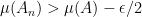${\mu(A_n)>\mu(A)-\epsilon/2}$ . As ${A_n\in\mathcal B}$ , there exists ${B\subseteq A_n}$ in ${\mathcal A_\delta}$ such that ${\mu(B)>\mu(A_n)-\epsilon/2}$ . Then, (1) holds and, hence, A is in ${\mathcal B}$ .

Now consider a sequence ${A_n\in\mathcal B}$ decreasing to the limit A. For each n, choose ${B_n\subseteq A_n}$ in ${\mathcal A_\delta}$ such that ${\mu(B_n) > \mu(A_n)-2^{-n}\epsilon}$ . Then, setting ${B=\bigcap_nB_n\in\mathcal A_\delta}$ ,

$\displaystyle \setlength\arraycolsep{2pt} \begin{array}{rl} \displaystyle\mu(A\setminus B)&\displaystyle= \mu\left(\bigcap\nolimits_nA_n\setminus\bigcap\nolimits_nB_n\right)\smallskip\\ &\displaystyle\le\mu\left(\bigcup\nolimits_n(A_n\setminus B_n)\right)\smallskip\\ &\displaystyle < \sum_n2^{-n}\epsilon=\epsilon. \end{array}$

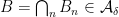So, (1) is satisfied, and ${A\in\mathcal B}$ . We have shown that ${\mathcal B}$ is closed under taking limits of increasing and decreasing sequences, and the monotone class theorem gives ${\mathcal B=\mathcal E}$ . ⬜

We put together the previous two lemmas to state and prove the generalised section theorem. This is the point where measurable section will be required, in order to be able to apply the previous lemma. A minor technicality is that, if we do not assume completeness of the probability space, the projection ${\pi_\Omega(S)}$ need not be measurable and so need not be in the domain ${\mathcal F}$ of the probability measure ${{\mathbb P}}$ . To get around this, we use the outer measure

$\displaystyle {\mathbb P}^*(A)\equiv\inf\left\{{\mathbb P}(B)\colon B\in\mathcal F, B\supseteq A\right\}$

which is defined on all subsets of ${\Omega}$ .

Theorem 3 (Generalised Section Theorem) Let ${\mathcal T}$ be a collection of random times defined on a probability space ${(\Omega,\mathcal F,{\mathbb P})}$ and satisfying the conditions of lemma 1, and let ${\mathcal E}$ be the sigma-algebra on ${\Omega\times{\mathbb R}^+}$ ,

$\displaystyle \mathcal E=\sigma\left([\tau,\infty)\colon\tau\in\mathcal T\right).$

Then, for any ${S\in\mathcal E}$ and ${\epsilon > 0}$ , there exists a ${\tau\in\mathcal T}$ satisfying ${[\tau]\subseteq S}$ and,

$\displaystyle {\mathbb P}(\tau < \infty) > {\mathbb P}^*(\pi_\Omega(S))-\epsilon.$

Proof: Let ${\mathcal A}$ be the collection of finite unions of stochastic intervals ${[\sigma,\tau)}$ over ${\sigma,\tau\in\mathcal T}$ . By lemma 1 this is an algebra on ${\Omega\times{\mathbb R}^+}$ . As

$\displaystyle [\sigma,\tau)=[\sigma,\infty)\setminus[\tau,\infty),$

the sigma-algebra ${\sigma(\mathcal A)}$ is also generated by the stochastic intervals ${[\tau,\infty)}$ over ${\tau\in\mathcal T}$ , so is equal to ${\mathcal E}$ .

The idea is to use lemma 2 in order to approximate ${S\in\mathcal E}$ from below by some ${A\in\mathcal A_\delta}$ , which requires defining a measure ${\mu}$ on ${(\Omega\times{\mathbb R}^+,\mathcal E)}$ . This is where we make use of the measurable section theorem, which states that there exists a random time ${\sigma\colon\Omega\rightarrow\bar{\mathbb R}^+}$ satisfying ${[\sigma]\subseteq S}$ and ${{\mathbb P}(\sigma < \infty)={\mathbb P}^*(\pi_\Omega(S))}$ . A measure ${\mu}$ can then be defined by

$\displaystyle \setlength\arraycolsep{2pt} \begin{array}{rl} \displaystyle\mu(A)&\displaystyle={\mathbb P}\left(\sigma\in A\right)\equiv{\mathbb P}\left(\{\omega\in\Omega\colon(\omega,\sigma(\omega))\in A\}\right)\smallskip\\ &\displaystyle\le{\mathbb P}^*\left(\pi_\Omega(A)\right) \end{array}$

for ${A\in\mathcal E}$ . This satisfies ${\mu(S)={\mathbb P}^*(\pi_\Omega(S))}$ and lemma 2 states that there is an ${A\subseteq S}$ in ${\mathcal A_\delta}$ with

$\displaystyle {\mathbb P}^*(\pi_\Omega(A))\ge \mu(A) > {\mathbb P}^*(S) - \epsilon.$

Lemma 1 now gives a ${\tau\in\mathcal T}$ with

$\displaystyle [\tau]\subseteq[D(A)]\subseteq A\subseteq S$

and ${\tau = D(A)}$ almost surely. So,

$\displaystyle \setlength\arraycolsep{2pt} \begin{array}{rl} \displaystyle{\mathbb P}(\tau < \infty) &\displaystyle= {\mathbb P}^*(D(A) < \infty)\smallskip\\ &\displaystyle={\mathbb P}^*(\pi_\Omega(A))\smallskip\\ &\displaystyle > {\mathbb P}^*(\pi_\Omega(S))-\epsilon \end{array}$

as required. ⬜

Optional Section

Recall that a filtration ${\{\mathcal F_t\}_{t\in{\mathbb R}^+}}$ on a probability space ${(\Omega,\mathcal F,{\mathbb P})}$ is a collection of sub-sigma-algebras ${\mathcal F_t\subseteq\mathcal F}$ which is increasing in t, so ${\mathcal F_s\subseteq F_t}$ for ${s\le t}$ . Taken together, this defines a filtered probability space ${(\Omega,\mathcal{F},\{\mathcal{F}_t\}_{t\in{\mathbb R}^+},{\mathbb P})}$ . It is common to assume the usual conditions that the probability space is complete, ${\mathcal F_0}$ contains all zero probability sets and that the filtration is right-continuous. We do not do this here, and will not assume any conditions other than the existence of the filtered probability space.

A stopping time is a random time ${\tau\colon\Omega\rightarrow\bar{\mathbb R}^+}$ such that

$\displaystyle \{\tau\le t\}\in\mathcal F_t$

for all times ${t\in{\mathbb R}^+}$ . Defining the optional sigma-algebra on ${\Omega\times{\mathbb R}^+}$ ,

$\displaystyle \mathcal O=\sigma\left([\tau,\infty)\colon\tau{\rm\ is\ a\ stopping\ time}\right),$

the optional section theorem is as follows.

Theorem 4 (Optional Section) For any ${S\in\mathcal O}$ and ${\epsilon > 0}$ , there exists a stopping time ${\tau}$ with ${[\tau]\subseteq S}$ and

$\displaystyle {\mathbb P}(\tau < \infty) > {\mathbb P}^*(\pi_\Omega(S))-\epsilon.$

Proof: It just needs to be shown that the collection, ${\mathcal T}$ , of all stopping times satisfies the conditions of lemma 1. The result will then follow from generalised section, theorem 3, above.

Starting with ${\sigma,\tau\in\mathcal T}$ and ${t\in{\mathbb R}^+}$ ,

$\displaystyle \setlength\arraycolsep{2pt} \begin{array}{rl} \displaystyle\{\sigma\wedge\tau\le t\}&\displaystyle=\{\sigma\le t\}\cup\{\tau\le t\},\smallskip\\ \displaystyle\{\sigma_{\{\sigma < \tau\}}\le t\}&\displaystyle=\{\sigma\le t, \sigma < \tau\}\smallskip\\ &\displaystyle=\bigcup_{s\in S}(\{\sigma\le s\}\setminus\{\tau\le s\}) \end{array}$

where S is any countable dense subset of ${[0,t]}$ with ${t\in S}$ . These sets are in ${\mathcal F_t}$ , showing that ${\sigma\wedge\tau}$ and ${\sigma_{\{\sigma < \tau\}}}$ are stopping times. Similarly, if ${\tau_n}$ is a sequence of stopping times then,

$\displaystyle \{\sup\nolimits_n\tau_n\le t\}=\bigcap_{n=1}^\infty\{\tau_n\le t\}$

is in ${\mathcal F_t}$ , so ${\sup_n\tau_n}$ is a stopping time. ⬜

Predictable Section

We continue to work with respect to the filtered probability space ${(\Omega,\mathcal{F},\{\mathcal{F}_t\}_{t\in{\mathbb R}^+},{\mathbb P})}$ . A map ${\tau\colon\Omega\rightarrow\bar{\mathbb R}^+}$ is called a predictable stopping time if there exists a sequence of stopping times ${\tau_n}$ increasing to ${\tau}$ and satisfying ${\tau_n < \tau}$ whenever ${\tau\not=0}$ . The sequence ${\tau_n}$ is said to announce ${\tau}$ and, as ${\tau=\sup_n\tau_n}$ , predictable stopping times are always stopping times. The conditions are required to hold pointwise on ${\Omega}$ , so that ${\tau_n(\omega)}$ announces ${\tau(\omega)}$ everywhere on ${\Omega}$ . For brevity, I will also use predictable time to refer to predictable stopping times.

The predictable sigma-algebra on ${\Omega\times{\mathbb R}^+}$ is defined by

$\displaystyle \mathcal P=\sigma\left([\tau,\infty)\colon\tau{\rm\ is\ a\ predictable\ stopping\ time}\right).$

Ideally, we would like to proceed in just the same way as we did above for the optional section theorem, and show that the collection of predictable times satisfies all of the required properties to apply generalised section, theorem 3. Although they very nearly satisfy the requirements, unfortunately it does not quite work. The time ${\sigma_{\{\sigma < \tau\}}}$ need not be predictable even when ${\sigma}$ and ${\tau}$ are predictable, although it is almost surely equal to a predictable stopping time.

Lemma 5 The collection of predictable stopping times satisfies,

${\sup_n\tau_n}$ is a predictable stopping time, for all sequences ${\tau_1,\tau_2,\ldots}$ of predictable stopping times.
for predictable stopping times ${\sigma}$ and ${\tau}$ ,

${\sigma\wedge\tau}$ is a predictable stopping time.
there exists a predictable stopping time ${\upsilon\le\sigma_{\{\sigma < \tau\}}}$ with ${\upsilon=\sigma_{\{\sigma < \tau\}}}$ almost surely.
for any ${\epsilon > 0}$ there exists a predictable stopping time ${\upsilon\ge\sigma_{\{\sigma < \tau\}}}$ with ${{\mathbb P}(\upsilon\not=\sigma_{\{\sigma < \tau\}}) < \epsilon}$ .

Proof: Before proceeding with the proof, recall that ${\tau_n\uparrow\tau}$ announces ${\tau}$ if ${\tau_n < \tau}$ whenever ${\tau\not=0}$ . In what follows, it is convenient to relax this condition slightly so that ${\tau_n < \tau}$ whenever ${\tau\not\in\{0,\infty\}}$ . It is still be the case that ${n\wedge\tau_n}$ announces ${\tau}$ in the sense defined above and that ${\tau}$ is predictable.

If each ${\tau_n}$ ( ${n\in{\mathbb N}}$ ) is announced by the stopping times ${\tau_{n1},\tau_{n2},\ldots}$ , then it follows that the stopping times

$\displaystyle \tau^\prime_n\equiv\tau_{n1}\vee\tau_{n2}\vee\cdots\vee\tau_{nn}$

announce ${\sup_n\tau_n}$ which, therefore, is a predictable stopping time.

Now, let ${\sigma,\tau}$ be announced, respectively, by the sequences ${\sigma_n}$ and ${\tau_n}$ of stopping times. Clearly, ${\sigma_n\wedge\tau_n}$ announces ${\sigma\wedge\tau}$ which, hence, is a predictable stopping time. Next, fix an ${m\in{\mathbb N}}$ and consider the stopping times

$\displaystyle \upsilon_n\equiv(\sigma_n)_{\{\sigma_n < \tau_m\}}.$

These announce ${\sigma}$ whenever ${\tau_m}$ is positive and ${\sigma\le\tau_m}$ , and are eventually infinite otherwise. So, they announce ${\upsilon\equiv\sigma_{\{\sigma\le\tau_m\not=0\}}}$ which is, therefore, a stopping time. By construction, ${\upsilon\ge\sigma_{\{\sigma < \tau\}}}$ and,

$\displaystyle \setlength\arraycolsep{2pt} \begin{array}{rl} \displaystyle{\mathbb P}\left(\upsilon\not=\sigma_{\{\sigma < \tau\}}\right)&\displaystyle={\mathbb P}\left(\{\sigma < \tau\}\setminus\{\sigma\le\tau_m\not=0\}\right)\smallskip\\ &\displaystyle\le {\mathbb P}\left(\tau_m \le \sigma < \tau\right). \end{array}$

By monotone convergence, this tends to zero as m goes to infinity, so can be made less that any given ${\epsilon > 0}$ , proving the final statement of the lemma.

Finally, we show that ${\sigma_{\{\sigma < \tau\}}}$ is almost surely equal to a predictable time. This will make use of the Borel-Cantelli lemma to construct a sequence of stopping times which almost surely announces ${\sigma_{\{\sigma < \tau\}}}$ . Start by choosing a sequence ${n_1,n_2,\ldots\in{\mathbb N}}$ and define the times,

$\displaystyle \upsilon_k=\inf\{\sigma_{n_j}\colon j\ge k, \sigma_{n_j} < \tau_j\}.$

These are stopping times, as we see by writing

$\displaystyle \{\upsilon_k\le t\}=\bigcup_{j\ge k}\left\{(\sigma_{n_j})_{\{\sigma_{n_j} < \tau_j\}}\le t\right\}$

If we let A be the event that ${\sigma_{n_k} < \tau_k}$ infinitely often, then it can be seen that ${\upsilon_k}$ announces ${\sigma_A}$ which, therefore, is a predictable stopping time. Whenever ${\sigma < \tau}$ , we have ${\tau_k > \sigma\ge\sigma_{n_k}}$ for large k, so ${\{\sigma < \tau\}\subseteq A}$ and hence, ${\sigma_A\le\sigma_{\{\sigma < \tau\}}}$ .

It only remains to show that ${\sigma_A=\sigma_{\{\sigma < \tau\}}}$ almost surely. For each k, ${n_k}$ can be chosen large enough so that

$\displaystyle {\mathbb P}(\sigma_{n_k} < \tau_k\le\sigma) < 2^{-k}.$

On the event ${\{\sigma\ge\tau\}}$ we have ${\tau_k\le\sigma}$ so, from Borel-Cantelli, ${\sigma_{n_k}\ge\tau_k}$ for large k, almost surely. This means that, up to a zero probability event, ${A\subseteq\{\sigma < \tau\}}$ and, hence, ${\sigma_{\{\sigma < \tau\}}\le\sigma_A}$ as required. ⬜

There are several ways around the issue that ${\sigma_{\{\sigma < \tau\}}}$ need not be predictable. Lemma 5 shows that it is almost surely predictable. If we were to modify the definition of predictable stopping times so that the sequence ${\tau_n}$ is only required to announce ${\tau}$ almost surely, then the problem goes away. However, the definition of stopping times, predictable stopping times, and of the optional and predictable sigma algebras do not make reference to the probability measure ${{\mathbb P}}$ at all, and we would prefer to keep it this way. Another approach, which amounts to the same thing, is to assume further properties of the filtration, specifically that ${\mathcal F_0}$ contains all zero probability sets. We would prefer not to add further preconditions to the section theorem if they are not necessary. Another approach, taken by Dellacherie & Meyer (Probabilities and Potential, A, 1979) is to first define the predictable sigma-algebra, and then say that a stopping time ${\tau}$ is predictable if its graph ${[\tau]}$ is in ${\mathcal P}$ . This also works, and such times can be shown to be announced in an almost sure sense, but we would prefer to work with the stronger and more intuitive definition given above. In fact, the predictable section theorem does hold without any such modification to the definition of predictable stopping times, and without requiring any further preconditions.

Theorem 6 (Predictable Section) For any ${S\in\mathcal P}$ and ${\epsilon > 0}$ , there exists a predictable stopping time ${\tau}$ with ${[\tau]\subseteq S}$ and

$\displaystyle {\mathbb P}(\tau < \infty) > {\mathbb P}^*(\pi_\Omega(S))-\epsilon.$

Proof: As noted above, we cannot simply let ${\mathcal T}$ be the collection of predictable times and apply theorem 3. The problem is that, if ${\sigma,\tau}$ are in ${\mathcal T}$ , then it does not necessarily follow that ${\sigma_{\{\sigma < \tau\}}}$ is in ${\mathcal T}$ .

Instead, we let ${\mathcal T}$ be the collection of stopping times ${\tau\colon\Omega\rightarrow\bar{\mathbb R}^+}$ such that, for all ${\epsilon > 0}$ , there exists predictable stopping times ${\upsilon}$ and ${\nu}$ satisfying ${\upsilon\le\tau\le\nu}$ and ${{\mathbb P}(\upsilon\not=\nu) < \epsilon}$ . We show that this does satisfy the requirements stated in lemma 1.

Considering a sequence ${\tau_n\in\mathcal T}$ and choosing ${\epsilon > 0}$ , there exists predictable times ${\upsilon_n\le\tau_n\le\nu_n}$ satisfying ${{\mathbb P}(\upsilon_n\not=\nu_n) < 2^{-n}\epsilon}$ . Then,

$\displaystyle \upsilon\equiv\sup_n\upsilon_n\le\tau\equiv\sup_n\tau_n\le\nu\equiv\sup_n\nu_n$

and lemma 5 says that ${\upsilon,\nu}$ are predictable. Writing,

$\displaystyle \setlength\arraycolsep{2pt} \begin{array}{rl} \displaystyle{\mathbb P}\left(\upsilon\not=\nu\right) &\displaystyle\le {\mathbb P}\left(\exists n, \upsilon_n\not=\nu_n \right)\smallskip\\ &\displaystyle < \sum_n2^{-n}\epsilon = \epsilon, \end{array}$

shows that ${\tau\in\mathcal T}$ as required.

Now consider ${\sigma,\tau\in\mathcal T}$ , choose ${\epsilon > 0}$ , so that there exists predictable times ${\sigma_1\le\sigma\le\sigma_2}$ and ${\tau_1\le\tau\le\tau_2}$ with

$\displaystyle {\mathbb P}(\sigma_1\not=\sigma_2) < \epsilon/3,\ {\mathbb P}(\tau_1\not=\tau_2) < \epsilon/3.$

Lemma 5 says that ${\upsilon,\nu}$ are predictable where,

$\displaystyle \upsilon\equiv\sigma_1\wedge\tau_1\le(\sigma\wedge\tau)\le\nu\equiv\sigma_2\wedge\tau_2.$

Then,

$\displaystyle {\mathbb P}\left(\upsilon\not=\nu\right) \le{\mathbb P}\left(\sigma_1\not=\sigma_2{\rm\ or\ }\tau_1\not=\tau_2\right) < \epsilon$

shows that ${\sigma\wedge\tau\in\mathcal T}$ . Next, lemma 5 says that there are predictable stopping times ${\upsilon,\nu}$ satisfying

$\displaystyle \upsilon\le(\sigma_1)_{\{\sigma_1 < \tau_2\}}\le\sigma_{\{\sigma < \tau\}}\le(\sigma_2)_{\{\sigma_2 < \tau_1\}}\le\nu$

and with ${\upsilon=(\sigma_1)_{\{\sigma_1 < \tau_2\}}}$ almost surely, and ${{\mathbb P}(\nu\not=(\sigma_2)_{\{\sigma_2 < \tau_1\}}) < \epsilon/3}$ . Then,

$\displaystyle {\mathbb P}(\upsilon\not=\nu)\le{\mathbb P}\left(\sigma_1\not=\sigma_2{\rm\ or\ }\tau_1\not=\tau_2{\rm\ or\ }(\sigma_2)_{\{\sigma_2 < \tau_1\}}\not=\nu\right) < \epsilon$

showing that ${\sigma_{\{\sigma < \tau\}}\in\mathcal T}$ .

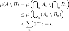
We have shown that ${\mathcal T}$ satisfies all the required properties for generalised section, theorem 3, to apply. As every predictable stopping time is in ${\mathcal T}$ , this means that for any predictable set ${S\in\mathcal P}$ and ${\epsilon > 0}$ , there exists a time ${\sigma\in\mathcal T}$ with ${[\sigma]\subseteq S}$ and

$\displaystyle {\mathbb P}(\sigma < \infty) > {\mathbb P}^*(\pi_\Omega(S))-\epsilon/2.$

Also, by definition of ${\mathcal T}$ , there is a predictable time ${\tau\ge\sigma}$ with ${{\mathbb P}(\tau\not=\sigma) < \epsilon / 2}$ . If ${\tau_n}$ are stopping times announcing ${\tau}$ , then ${(\tau_n)_{\{\tau_n\le\sigma\}}}$ announces ${\tau_{\{\tau=\sigma\}}}$ ,

$\displaystyle \setlength\arraycolsep{2pt} \begin{array}{rl} &\displaystyle[\tau_{\{\tau=\sigma\}}]\subseteq[\sigma]\subseteq S,\smallskip\\ &\displaystyle{\mathbb P}(\tau_{\{\tau=\sigma\}} < \infty)\ge{\mathbb P}(\tau=\sigma < \infty) > {\mathbb P}^*\left(\pi_\Omega(S)\right) - \epsilon \end{array}$

as required. ⬜

3 thoughts on “Proof of Optional and Predictable Section”

Matti Kiiski says:

14 December 19 at 10:39 PM

Dear George,

I noticed that there is a missing subscript $n$ in the definition of the slices $S_n(\omega)$ . Also, it is unclear at that point that $S_n$ is a sequence coming from the family $\mathcal A$ .

Also, I would like to remark that a generalized version of section theorem is sometimes called “Meyer section theorem”. Accordingly, the projections then generalize to the so-called “Meyer $\sigma$ -algebras”; see Lenglart (1980) and El Karoui (1981).

Thank you for another great post and all the best.

1. George Lowther says:
  
  15 December 19 at 4:24 PM
  
  Thanks, I’ll update the post when I have a few moments. Also, I fixed your latex, which should start $latex.
  Regards
  
  1. Matti Kiiski says:
    
    16 December 19 at 5:03 PM
    
    Thank you very much. I also forgot to include the names of the papers. Here are they:
    
    E. Lenglart. Tribus de Meyer et théorie des processus, volume 784 of Lecture Notes in Math. Springer, Berlin, 1980.
    
    N. El Karoui. Les aspects probabilistes du contrôle stochastique. In Ninth Saint Flour Probability Summer School—1979 (Saint Flour, 1979), volume 876 of Lecture Notes in Math., pages 73–238. Springer, Berlin-New York, 1981.
    
    With best regards

	Tavin on Class (D) Processes
	George Lowther on Filtrations and Adapted P…
	faceet on Filtrations and Adapted P…
	George Lowther on Filtrations and Adapted P…
	facet on Filtrations and Adapted P…
	Zoltan on Class (D) Processes
	Zoltan on Class (D) Processes
	ARS on Stopping Times and the Debut…
	George Lowther on Upcrossings, Downcrossings, an…
	George Lowther on Stopping Times and the Debut…

Proof of Optional and Predictable Section

Optional Section

Predictable Section

Published by George Lowther

3 thoughts on “Proof of Optional and Predictable Section”

Leave a Reply Cancel reply

Optional Section

Predictable Section

Like this:

Related

Published by George Lowther

3 thoughts on “Proof of Optional and Predictable Section”

Leave a Reply Cancel reply