The aim of this post is to give a direct proof of the theorems of measurable projection and measurable section. These are generally regarded as rather difficult results, and proofs often use ideas from descriptive set theory such as analytic sets. I did previously post a proof along those lines on this blog. However, the results can be obtained in a more direct way, which is the purpose of this post. Here, I present relatively self-contained proofs which do not require knowledge of any advanced topics beyond basic probability theory.
The projection theorem states that if is a complete probability space, then the projection of a measurable subset of onto is measurable. To be precise, the condition is that S is in the product sigma-algebra , where denotes the Borel sets in , and the projection map is denoted
Then, measurable projection states that . Although it looks like a very basic property of measurable sets, maybe even obvious, measurable projection is a surprisingly difficult result to prove. In fact, the requirement that the probability space is complete is necessary and, if it is dropped, then need not be measurable. Counterexamples exist for commonly used measurable spaces such as and . This suggests that there is something deeper going on here than basic manipulations of measurable sets.
By definition, if then, for every , there exists a such that . The measurable section theorem — also known as measurable selection — says that this choice can be made in a measurable way. That is, if S is in then there is a measurable section,
It is convenient to extend to the whole of by setting outside of .
Figure 1: A section of a measurable set
The graph of is
The condition that whenever can alternatively be expressed by stating that . This also ensures that is a subset of , and is a section of S on the whole of if and only if .
The results described here can also be used to prove the optional and predictable section theorems which, at first appearances, also seem to be quite basic statements. The section theorems are fundamental to the powerful and interesting theory of optional and predictable projection which is, consequently, generally considered to be a hard part of stochastic calculus. In fact, the projection and section theorems are really not that hard to prove.
Let us consider how one might try and approach a proof of the projection theorem. As with many statements regarding measurable sets, we could try and prove the result first for certain simple sets, and then generalise to measurable sets by use of the monotone class theorem or similar. For example, let denote the collection of all for which . It is straightforward to show that any finite union of sets of the form for and are in . If it could be shown that is closed under taking limits of increasing and decreasing sequences of sets, then the result would follow from the monotone class theorem. Increasing sequences are easily handled — if is a sequence of subsets of then from the definition of the projection map,
If for each n, this shows that the union is again in . Unfortunately, decreasing sequences are much more problematic. If for all then we would like to use something like
(1)
However, this identity does not hold in general. For example, consider the decreasing sequence . Then, for all n, but is empty, contradicting (1). There is some interesting history involved here. In a paper published in 1905, Henri Lebesgue claimed that the projection of a Borel subset of onto is itself measurable. This was based upon mistakenly applying (1). The error was spotted in around 1917 by Mikhail Suslin, who realised that the projection need not be Borel, and lead him to develop the theory of analytic sets.
Actually, there is at least one situation where (1) can be shown to hold. Suppose that for each , the slices
(2)
are compact. For each , the slices give a decreasing sequence of nonempty compact sets, so has nonempty intersection. So, letting S be the intersection , the slice is nonempty. Hence, , and (1) follows.
The starting point for our proof of the projection and section theorems is to consider certain special subsets of where the compactness argument, as just described, can be used. The notation is used to represent the collection of countable intersections, , of sets in .
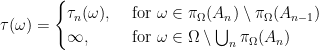
Lemma 1 Let be a measurable space, and be the collection of subsets of which are finite unions over compact intervals and . Then, for any , we have , and the debut
is a measurable map with and .
Proof: Noting that and the collection of compact intervals in are closed under pairwise intersection, the same is true for . Then, for there exists, by definition, such that . Replacing by if necessary, we may suppose that is a decreasing sequence.
Now, the slices defined by (2) are finite unions of compact intervals, so are compact. The compactness argument explained above implies that
(3)
As each is a finite union for and nonempty , the projection is in . Then, (3) shows that is also in .
If is the debut of S, then . This immediately implies and, as nonempty compact sets contain their infimum, . For every , the set is in and,
showing that is measurable. ⬜
When dealing with more general subsets of , it will not necessarily be the case that the projection onto is measurable. For that reason, we extend the probability measure to more general subsets of . For a probability space , define an outer measure on the power set by approximating from above by measurable sets,
(4)
The outer measure has the following basic properties.
Lemma 2 For a probability space , the outer measure is increasing and continuous along increasing sequences. That is, for , and for sequences increasing to a limit A.
Furthermore, for any , there exists in with .
Proof: The fact that is increasing is immediate from the definition. Now, let be increasing to the limit A. By the definition of , there exists in with
Replacing by if necessary, we may suppose that is an increasing sequence. Then, is in and, by monotone convergence,
So, as required. Incidentally, this also shows that there is a in with . ⬜
I now move on the the main component of the proof of the projection and section theorems. This will allow us to approximate measurable subsets of from below by sets in , as defined in lemma 1 above. While the statement of theorem 3 is simple enough, the proof can get a bit tricky. The method used here is elementary and, although the argument is a bit intricate, no advanced mathematics is required. The definition of means that it is the minimal collection of subsets of X which contains and is closed under taking limits of increasing and decreasing sequences. I refer to the result as the `capacitability theorem’ as it is a version of Choquet’s capacitability theorem although, here, we do not involve the concept of analytic sets. A set can be called capacitable if, for each , there exists a decreasing sequence with and . So, theorem 3 is saying that all sets in are capacitable.
Theorem 3 (Capacitability Theorem) Let X be a set, be closed under pairwise intersections, and be increasing and continuous along increasing sequences. Denote the closure of under limits of increasing and of decreasing sequences by .
Then, for any and with , there exists a decreasing sequence with and for all n.
Proof: Fixing , let denote the collection of all with . The assumptions on I mean that for any then every is in and, for any sequence increasing to A, then for large n.
The proof of the theorem amounts to finding a collection containing and closed under taking limits of increasing and decreasing sequences, such that, for every , we can construct a decreasing sequence with . In that case, every will also be in , and the claimed result will follow.
The main difficulty in the proof is to describe a collection with the required properties. One way of doing this is as follows, and can be described in terms of a game. For , consider the following infinite game played between two players, who take turns choosing sets from . Starting with , at rounds , the players make the following moves.
Player 1 chooses an in .
Player 2 chooses a in .
At each round, both players can, at least, make a valid move. For example, player 1 can set and player 2 can set . We say that player 2 wins the game if, once completed, she is able to find a sequence in with .
For any , denote the game described above by . A strategy (for player 2) is just a sequence of functions satisfying
(5)
The idea is that represents player 2’s choice for at round n, given that player 1 has chosen so far. It is a winning strategy if, for any sequence satisfying
(6)
for each , then there exists a sequence with
(7)
We note that, combining (5) and (6) shows that must be a decreasing sequence of subsets of A.
Now, let be the collection of for which the game has a winning strategy. The case with is easy. Any strategy is a winning strategy simply by taking in (7). For we may as well take , which is a valid strategy.
Now, consider a sequence and let be winning strategies for . Construct a winning strategy for , with , as follows. Choose a bijection such that is increasing in s. For example, take . Then for and , define
It can be seen that this is a winning strategy. If (6) is satisfied then, writing , we use the fact that the sequence is decreasing and to write
for any . So, (6) is also satisfied for the sequence (for the strategy and game ). As is a winning strategy for , there exists in satisfying . In particular, writing gives
If is increasing, construct a winning strategy for as follows. For any with , the sequence increases to . Hence, there is a minimum r such that . Set,
For then we do not really care, so can just take . This clearly gives a valid strategy. To see that it is a winning strategy, suppose that (6) is satisfied. Setting and for , we see that (6) is also satisfied with in place of and in place of . So, as is a winning strategy for the game , there exists a sequence with
So, is a winning strategy for and, hence, .
We have shown that contains and is closed under taking limits of increasing and decreasing sequences and, so, contains . Finally, for any , let be a winning strategy for and define a sequence by and
for all . As is a winning strategy, there exists a sequence satisfying (7). Replacing by if required, we can suppose that the sequence is decreasing. Finally, as , we have as required. ⬜
The argument above is along similar lines to the `rabotages de Sierpinski’ used by Dellacherie, Ensembles aléatoires II (1969). Although the description of the collection in terms of winning strategies of the games may not seem like an obvious approach, it is really quite natural. As a first attempt to prove the result, we could try defining to be the collection of sets for which the conclusion of the theorem holds. That is, the sets A for which there is a decreasing sequence with . We would then have to show that is closed under taking limits of increasing and decreasing sequences. While increasing sequences are easy to deal with, decreasing ones are problematic. Suppose that decreases to A and that, for each n, there is a decreasing sequence with . To construct a sequence of sets we could try to do the following. Reorder the doubly-indexed sequence into a singly-indexed one, and set . Then, it is clear that and . However, is not decreasing. We could try and ensure that it is decreasing by setting
Unfortunately, it is no longer necessarily true that is in . When we take intersections we need no longer be in . The easiest way around this, it seems, is to allow the choice of to depend on the previous choices of . That is, the choice of should depend on so as to enforce the condition that is in . This leads, essentially, to the requirement of winning strategies for the games as described in the proof of theorem 3.
We use theorem 3 to show that measurable subsets of can be approximated from below by .
Corollary 4 Let be a probability space and be the collection of subsets of given in lemma 1. Then, for any and , there exists in satisfying
Proof: Setting , define
This is clearly increasing. Also, if is increasing to a limit A then increases to . Lemma 2 implies that , and I is continuous along increasing sequences.
As the complement of a compact interval in is a countable union of compact intervals, the complement of any is a countable union of . The monotone class theorem then says that the closure of under limits of increasing and decreasing sequences is the entire sigma-algebra generated by . Hence,
We apply theorem 3. For and , setting , there exists a decreasing sequence with and . Take which is in . As in the proof of lemma 1, decreases to . By monotone convergence,
as required. ⬜
Combining this result with the statement, in lemma 1, of measurable projection for sets in gives the measurable projection theorem.
Theorem 5 (Measurable Projection) Let be a complete probability space, and . Then, .
Proof: By corollary 4, for each positive integer n, there is an in with
(8)
We know from lemma 1 that are measurable, so is in , is contained in , and satisfies . Lemma 2 states that there is a in and satisfying .
We have constructed sets in and satisfying . By definition, this means that is in the completion of and, if the probability space is complete, it is in . ⬜
In a similar way, corollary 4 combined with the statement of measurable section for sets in , given by lemma 1, gives the measurable section theorem.
Theorem 6 (Measurable Section) Let be a probability space and . Then, there exists a measurable , such that and is -null.
Proof: As in the proof of theorem 5, there is a sequence in satisfying (8). Replacing by if necessary, we suppose that the sequence is increasing. Let be the debut of , Lemma 1 states that this is measurable and . Define a random time by,
(I am using ). This is measurable with graph contained in S and,
By lemma 2, there exists containing with . So, has zero probability and contains , which is -null as required. ⬜
Finally, we state the theorem for complete probability spaces, in which case the section is defined on all of , and not just up to a -null set.
Theorem 7 (Measurable Section) Let be a complete probability space and . Then, there exists a measurable , such that and .
Proof: By theorem 6 there exists a measurable map such that and is -null. Define by
Here, represents the slice of S defined as in (2). We do not care about which t is chosen in the third case but, as is nonempty on , a choice does exist. By construction, , , and almost surely. As is measurable, completeness of the probability space implies that is also measurable. ⬜
33 thoughts on “Proof of the Measurable Projection and Section Theorems”
Hi the formalization of is a little confusing to me. Do you mean something like the following ?
For we set : , such that
In which case the “measurability” of is not completely clear to me.
Moreover the graph seems also a little ambiguous as what arrows point to are and not (which are parts of unless mistaken).
I don’t follow what you are saying. In the second paragraph, is a map from (which is a subset of ) to . So, and . You seem to be suggesting that is an element of , rather than a subset, and that is a subset of instead of an element.
On reflection, maybe you are not suggesting that is an element of and it is just a typo in your comment. However, it still looks like you are suggesting that is a subset of , which is not the case.
As you spotted it’s a typo, I meant intead of sorry about that. Coming back to my point, maybe I was confused about this quote :
“…hat is, if is in then there is a measurable section, ”
So shouldn’t you write instead (as I understand your answer to my comment) ?
My second point in this regard is pointless and you can delete my other post. I also note that you make clear a “language abuse” shortly after all this when you write :
“For brevity, the statement above will also be expressed by writing .” But I think it’s a bit early at this stage in your post to use this convention.
Last let me correct you on one thing. It’s definitely not you who is happy to see me back (but I fill honored about that nevertheless so thanks), it is me indeed who is happy to see more posts from you on this amazing blog…, I have seen guys on MO forum who do not dare to quote and refer this blog in their papers as it is no “OK to refer a blog, but who can’t find in the literature equivalent theorems claimed and proved in such a clear and self contained manner… cela veut tout dire.
Ah, I fixed the typo which caused your confusion, but it probably occurs elsewhere, so will fix properly later. I’ll also reread through and consider your suggestion regarding the notation when I have some time to properly edit this. Thanks!
Last comment maybe would it be simpler to switch axis in your graph illustrating , as it’s a function of and not the other way around.Regards
Rather than changing the graph, maybe it would be better to change the order of the Cartesian products throughout. instead of . That would be consistent with earlier stochastic calculus posts.
Another point is the ambiguity on the notation of sets in the counterexample after equation (2) to illustrate the missing property needed for application of MCT. In some cases it’s a set in ( and shortly after it is in unless mistaken. Regards
I don’t think there’s ambiguity. is a subset of , whereas is a subset of .
I changed the order of all cartesian products. Let me know what you think – if it is better, I’ll update the other posts.
Sorry a few more remarks (I am reading your post very slowly as you can notice;-) ):
-In the end I think that it would be nice to formalize the notion of “section”, by a fully fledged “definition 1” .
-Using the in your definition (2) of is a bit hard to follow for me as it is easy to forget that it’s only a compact of when is used and a part of when is dropped.
-The end of the argumentation for the “compact” example could be detailed a little bit more I think, I quote it his part :
“For each , the slices $latex{S_n(\omega)}$ give a decreasing sequence of nonempty compact sets, so has nonempty intersection. So, letting be the intersection , the slice is nonempty. Hence, , and (1) follows.”
So you proved then the slice of the intersection , namely is nonempty (part of ) in the first part and this is OK for me. But then the fact that this proves that still need a little more clarification even if it might seem trivial to you. So for your last claim to be true, I think you need to prove the following property :
For all nonempty and , we have : .
Proof : , by definition of a slice if it’s not empty then for then so that . let’s take a look at the “contrapositive” (i.e. non ), if then there is no such that and and we are done. End of proof. Does that seems ok to you ?
Hi I am reading the proof of theorem 3 and I was wondering about the fact that maybe , at a fixed , some of the sets might not be valid, in the sense that even though the sequence is a winning strategy, it is only for admissible sets for the game . I don’t really see right now why this has to be the case . Regards
I think that it is admissible, but maybe I should add a couple of sentences clarifying that.
I added the clarification.
Great it’s clear to me now, sorry to be so invasive…
Hi, I realized something quite trivial but still confusing about the conditions of applicability of theorem 3. If for all then by the properties of it is also true that for all . But then there exists no for which the conclusion of the theorem is applicable. I can’t figure out if that means that the theorem holds for such a case or not, my intuition is that it still holds because in the implicit “if” in the beginning of the conclusions of the theorem is not fulfilled, the end of the claim has no meaning which also means as it’s not applicable that the theorem still holds true in full generality, another way less elegant is to discard such bad behaved collection in the condition of the theorem. Regards
Hi discussing the proof with a friend he has shown me an elementary argument under the conditions of the theorem of capacitability here it is. First the assertion is trivial by taking a constant sequence equal to . Now if is the limit of a decreasing sequence in then it is also trivial as the sequence is in and its intersection (i.e. its limit) is equal to . Last if is the limit of an increasing sequence in then by continuity of the capacity I, for N big enough we have so if we take the sequence $A’_n =A_N$ we are done unless mistaken as we have exhibited a sequence for elements of decreasing included in and in . I think we might have missed something but we couldn’t see were we went wrong. Regards
Hi again I am now almost sure that it has to do with the definition of “closure under increasing and decreasing sequences”. In the argument above it is supposed that it is two properties that considered one by one but not together so that every set of the closure is either the limit of a monotone sequence of . Under this assumption I think that the closure is not a “idempotent” operator which would be a bit odd (even if I don’t have an explicit counterexample). If we consider the “AND” as meaning that every monotone sequences of the closure itself are themselves in the closure then maybe it would be possible to define it as the minimal collection with the property that it includes and is “stable” by monotone sequence. Regards
Yes, that is correct. The argument you gave does not apply to decreasing limits of increasing limits, or increasing limits of decreasing limits of increasing limits of sets in , etc. In fact, by results on the Borel Hierarchy of sets, if is the compact subsets of the reals, then it is not idempotent. In fact, the operation of taking increasing and decreasing limits does not stabilise until you get to the first uncountable ordinal.
Thanks for your kind reply, I must confess that I begin to feel like a Russian troll farm on a reddit forum here …
Anyway as your point applies then to my remark above for the case of for all (which was not so lame after all), as for it to be true for all which I though was simple, we would need in fact transfinite induction to get the result as the monotone limits of sets are not enough to conclude that for all . At last, I would really pleased to have a reference that shows that we have strict inclusion between the collection of monotone limits of sets in and the closure . Once again best regards
Hi, I think I have finished to make my points, and it would be best now to delete all those comments of mine.
Dear George,
thank you for the awesome blogpost. Since we can apply Theorem 5 for every probability measure in Theorem 6 we can actually say that the projection of lies in the universal completion, i.e. the intersection of the completions w.r.t. all probability distributions. Do you know (or have any reference) if we then still have a universally measurable section (similar to Theorem 7)? If so could we then directly start with an S in the universal completion of the product space and then have a universally measurable projection and corresponding section?
If you had any comments or pointers on this that would be great.
Hi Rudolph, Yes, there is a universally measurable section theorem, exactly as you suggested! I mentioned this, without proof, in my earlier proof of measurable section (https://almostsure.wordpress.com/2019/01/02/proof-of-measurable-section/). For a reference, this is proved in Cohn, Measure Theory, Corollary 8.5.4. I believe the proofs above could also be modified to show this.
For everyone reading this I also found a reference for an even slightly more general version in Bogachev’s Measure Theory Corollary 6.9.12 (due to Leese):
a Souslin space (eg Polish), any measurable space and an analytic/Souslin-B subset of (eg any measurable set). Then: is Souslin-B in (thus universally measurable) and there exists a section that is measurable wrt the -algebra generated by Souslin-B sets (in particular universally measurable).
It would be nice if one could get rid of all the topological conditions and just work with universally measurable spaces, maps and subsets.
Hi Rudolph. Regarding the more general versions of measurable section, there are a few points worth mentioning. First, allowing X to be Souslin is not much more general, as there will exist an onto Borel map , allowing you to reduce the problem to the case . Similarly, if S is Souslin-B, then it will be the projection of a measurable . This allows you to transfer the problem to the Borel set . Then, as above, you can replace the Souslin space by . So, extending from measurable subsets of to Souslin-B subsets of for Souslin spaces is not a big step.
However, the fact that the section can be chosen measurable with respect to the sigma-algebra generated by the Souslin-B sets does seem to be a significant strengthening compared to the sigma-algebra of universally measurable sets. I do not know of any applications of this though.
The suggestion in your first comments that maybe S could be taken in the universal completion of does seem unlikely to be true. This is significantly harder to deal with than measurable or Souslin-B sets. Would the measurable section result hold even for S assumed to be the complement of a Souslin-B set, for example? I doubt it, but constructing counterexamples is difficult. The uncountable axiom of choice would probably be needed — at least if the base space is the reals together with the Borel sigma-algebra — as there are versions of set theory in which countable dependent choice holds but every subset of the reals is universally measurable (Solovay model). Unfortunately non-universally measurable sets (Vitali sets) constructed using the AOC are going to be difficult to describe as projections of universally measurable sets, precisely because they were constructed using the AOC. Actually, I would not be surprised if such statements turn out to be dependent on the underlying logical axioms used, and may be independent of ZFC or of ZF+dependent choice.
In fact, the answer to the following math.stackexchange question is relevant here, “Which sets are lebesgue measurable in ZFC?”.
In particular “From 𝖬𝖠 (plus ¬𝖢𝖧) it follows that every set of reals is Lebesgue measurable”. This suggests that, to show that the projection of a co-analytic set is Lebesgue measurable, requires Martin’s Axiom and that the Continuum Hypothesis is false.
Also, you cannot go much further up the projective hierarchy without requiring theories which are stronger than ZFC — “Nevertheless, you cannot go much further by restricting to 𝖹𝖥𝖢 consistencywise: Shelah showed that the measurability of the sets implies the existence of inaccessible cardinals in 𝐿.”
.
Dear George Lowther,
Excellent post, interesting stuff. I have a suggestion on the arranging of proof 3 (Capacitability Theorem). As you correctly mention after it, the problem with the decreasing sequences can be dealt with if we are more strict and demand the choice of to depend on . In order to model this we make the following definitions:\\ .\\
The rest of the proof can easily be transformed analogously with what you do, i think these approach makes it a bit tidier, what do you think.
You see the problem with the natural approach, as you mentioned, specifically was that when we merge the boubly-indexed sequence into a singly-indexed one with the help of function the new sequence stops being decreasing. But with the definition that I gave for we can do the same process just fine for the corresponding functions in order to construct the new sequence that we need for the set intersection. The reason of course is that there is no decreasing requirement for the sequences that appear in the definition of .
Sorry for the consecutive comments but I didn’t have time to write everything in one go. You mention after the proof of theorem 3 that we can begin our attempts by defining . But this definition is problematic from the start, because there is no guarantee that . We need a condition in the form of <> or equivalent <>. Thinking like this we quickly arrive to the following intuitive definition, \latex \mathcal{B}:= \{A \subseteq X: \forall \{C_n\}_{n \geq 1} \subseteq \mathcal{C} \text{decreasing, with} C_1 \subseteq A \exists \{A_n\}_{n \geq 1} \text{such that} C_n \subseteq A_n \forall n \geq 1 \text{and} \bigcap_{n \geq 1}A_n \subseteq A\}$. Unfortunately this doesn’t work either, the problem though lies in the increasing sequences instead of the decreasing ones. The usual merging process works fine with the decrasing, however in the increasing case we want something to guarantee that the subsequence of the union falls fast enough so that we can see it as a subsequence of one of its members. This is the purpose of the functions in my first comment, they are “speed” conditions.
P.S.
There is a typo in the definition of in my first comment, the sequence should be a subset of instead of just .
Dear George,
It seems I misspelled in the use of latex at my last comment, it would be nice if you can fix it so it would be readable. Also in the PS I confused the notation, what I wanted to say is should be a subset of .


![\displaystyle [\tau]=\left\{(t,\omega)\in{\mathbb R}\times\Omega\colon t=\tau(\omega)\right\}.](https://s0.wp.com/latex.php?latex=%5Cdisplaystyle++%5B%5Ctau%5D%3D%5Cleft%5C%7B%28t%2C%5Comega%29%5Cin%7B%5Cmathbb+R%7D%5Ctimes%5COmega%5Ccolon+t%3D%5Ctau%28%5Comega%29%5Cright%5C%7D.+&bg=ffffff&fg=000000&s=0&c=20201002)


![{[\tau]\subseteq S}](https://s0.wp.com/latex.php?latex=%7B%5B%5Ctau%5D%5Csubseteq+S%7D&bg=ffffff&fg=000000&s=0&c=20201002)


be a measurable space, and
over compact intervals
and
. Then, for any
, we have


![{((-\infty,t]\times\Omega)\cap S}](https://s0.wp.com/latex.php?latex=%7B%28%28-%5Cinfty%2Ct%5D%5Ctimes%5COmega%29%5Ccap+S%7D&bg=ffffff&fg=000000&s=0&c=20201002)
![\displaystyle \{\tau\le t\}=\pi_\Omega\left(((-\infty,t]\times\Omega)\cap S\right)\in\mathcal F,](https://s0.wp.com/latex.php?latex=%5Cdisplaystyle++%5C%7B%5Ctau%5Cle+t%5C%7D%3D%5Cpi_%5COmega%5Cleft%28%28%28-%5Cinfty%2Ct%5D%5Ctimes%5COmega%29%5Ccap+S%5Cright%29%5Cin%5Cmathcal+F%2C+&bg=ffffff&fg=000000&s=0&c=20201002)


is increasing and continuous along increasing sequences. That is,
for
, and
for sequences
increasing to a limit A.
in
.


be closed under pairwise intersections, and
be increasing and continuous along increasing sequences. Denote the closure of
and
with
, there exists a decreasing sequence
for all n.


in
in


and
, there exists
in


, such that
is
-null.


![{[\tau_n]\subseteq A_n}](https://s0.wp.com/latex.php?latex=%7B%5B%5Ctau_n%5D%5Csubseteq+A_n%7D&bg=ffffff&fg=000000&s=0&c=20201002)

![{[\tau]}](https://s0.wp.com/latex.php?latex=%7B%5B%5Ctau%5D%7D&bg=ffffff&fg=000000&s=0&c=20201002)


![{[\tau_0]\subseteq S}](https://s0.wp.com/latex.php?latex=%7B%5B%5Ctau_0%5D%5Csubseteq+S%7D&bg=ffffff&fg=000000&s=0&c=20201002)


Hi the formalization of is a little confusing to me. Do you mean something like the following ?
 we set :

 , such that
 is not completely clear to me.
 and not
  (which are parts of
  unless mistaken).
For
In which case the “measurability” of
Moreover the graph seems also a little ambiguous as what arrows point to are
I don’t follow what you are saying. In the second paragraph, is a map from
  (which is a subset of
  ) to
) to  . So,
. So,  and
and  . You seem to be suggesting that
  is an element of
  , rather than a subset, and that
  is a subset of
  instead of an element.
On reflection, maybe you are not suggesting that is an element of
  and it is just a typo in your comment. However, it still looks like you are suggesting that
  is a subset of
  , which is not the case.
As you spotted it’s a typo, I meant intead of
  sorry about that. Coming back to my point, maybe I was confused about this quote :
 is in
is in  then there is a measurable section,
  ”
”

 above will also be expressed by writing
  .” But I think it’s a bit early at this stage in your post to use this convention.
“…hat is, if
So shouldn’t you write instead (as I understand your answer to my comment) ?
My second point in this regard is pointless and you can delete my other post. I also note that you make clear a “language abuse” shortly after all this when you write :
“For brevity, the statement
Last let me correct you on one thing. It’s definitely not you who is happy to see me back (but I fill honored about that nevertheless so thanks), it is me indeed who is happy to see more posts from you on this amazing blog…, I have seen guys on MO forum who do not dare to quote and refer this blog in their papers as it is no “OK to refer a blog, but who can’t find in the literature equivalent theorems claimed and proved in such a clear and self contained manner… cela veut tout dire.
Ah, I fixed the typo which caused your confusion, but it probably occurs elsewhere, so will fix properly later. I’ll also reread through and consider your suggestion regarding the notation when I have some time to properly edit this. Thanks!
Last comment maybe would it be simpler to switch axis in your graph illustrating , as it’s a function of
  and not the other way around.Regards
Rather than changing the graph, maybe it would be better to change the order of the Cartesian products throughout. instead of
  . That would be consistent with earlier stochastic calculus posts.
Another point is the ambiguity on the notation of sets in the counterexample after equation (2) to illustrate the missing property needed for application of MCT. In some cases it’s a set in
  (
( and shortly after it is in
  unless mistaken. Regards
I don’t think there’s ambiguity. is a subset of
  , whereas
  is a subset of
  .
.
I changed the order of all cartesian products. Let me know what you think – if it is better, I’ll update the other posts.
Sorry a few more remarks (I am reading your post very slowly as you can notice;-) ): by a fully fledged “definition 1” .
-In the end I think that it would be nice to formalize the notion of “section”,
-Using the in your definition (2) of
  is a bit hard to follow for me as it is easy to forget that it’s only a compact of
  when
when  is used and a part of
  when
when  is dropped.
-You say that a decreasing sequence of compact that’s unless mistaken a theorem from Cantor, could be worth mentioning to be self contained :https://en.wikipedia.org/wiki/Cantor%27s_intersection_theorem
-The end of the argumentation for the “compact” example could be detailed a little bit more I think, I quote it his part : , the slices $latex{S_n(\omega)}$ give a decreasing sequence of nonempty compact sets, so has nonempty intersection. So, letting
  be the intersection
  , the slice
  is nonempty. Hence,
  , and (1) follows.”
 then the slice of the intersection
  , namely
  is nonempty (part of
  ) in the first part and this is OK for me. But then the fact that this proves that
  still need a little more clarification even if it might seem trivial to you. So for your last claim to be true, I think you need to prove the following property :
 and
and  , we have :
 .
.
 , by definition of a slice if it’s not empty then for
  then
then  so that
  .
.
 let’s take a look at the “contrapositive” (i.e. non
  ), if
), if  then there is no
  such that
  and
and  and we are done. End of proof. Does that seems ok to you ?
“For each
So you proved
For all nonempty
Proof :
Hi I am reading the proof of theorem 3 and I was wondering about the fact that maybe , at a fixed
  , some of the sets
  might not be valid, in the sense that even though the sequence
  is a winning strategy, it is only for admissible sets
  for the game
  . I don’t really see right now why this has to be the case . Regards
I think that it is admissible, but maybe I should add a couple of sentences clarifying that.
I added the clarification.
Great it’s clear to me now, sorry to be so invasive…
Hi, I realized something quite trivial but still confusing about the conditions of applicability of theorem 3. If for all
  then by the properties of
  it is also true that
  for all
  . But then there exists no
  for which the conclusion of the theorem is applicable. I can’t figure out if that means that the theorem holds for such a case or not, my intuition is that it still holds because in the implicit “if” in the beginning of the conclusions of the theorem is not fulfilled, the end of the claim has no meaning which also means as it’s not applicable that the theorem still holds true in full generality, another way less elegant is to discard such bad behaved collection
  in the condition of the theorem. Regards
Hi discussing the proof with a friend he has shown me an elementary argument under the conditions of the theorem of capacitability here it is. First the assertion is trivial by taking a constant sequence equal to
  . Now if
  is the limit of a decreasing sequence in
  then it is also trivial as the sequence
  is in
is in  and its intersection (i.e. its limit) is equal to
  . Last if
  is the limit of an increasing sequence in
  then by continuity of the capacity I, for N big enough we have
  so if we take the sequence $A’_n =A_N$ we are done unless mistaken as we have exhibited a sequence for elements of
  decreasing included in
  and in
  . I think we might have missed something but we couldn’t see were we went wrong. Regards
Hi again I am now almost sure that it has to do with the definition of “closure under increasing and decreasing sequences”. In the argument above it is supposed that it is two properties that considered one by one but not together so that every set of the closure is either the limit of a monotone sequence of . Under this assumption I think that the closure is not a “idempotent” operator which would be a bit odd (even if I don’t have an explicit counterexample). If we consider the “AND” as meaning that every monotone sequences of the closure itself are themselves in the closure then maybe it would be possible to define it as the minimal collection with the property that it includes
  and is “stable” by monotone sequence. Regards
Yes, that is correct. The argument you gave does not apply to decreasing limits of increasing limits, or increasing limits of decreasing limits of increasing limits of sets in , etc. In fact, by results on the Borel Hierarchy of sets, if
  is the compact subsets of the reals, then it is not idempotent. In fact, the operation of taking increasing and decreasing limits does not stabilise until you get to the first uncountable ordinal.
Thanks for your kind reply, I must confess that I begin to feel like a Russian troll farm on a reddit forum here … for all
  (which was not so lame after all), as for it to be true for all
  which I though was simple, we would need in fact transfinite induction to get the result as the monotone limits of sets
  are not enough to conclude that
  for all
  . At last, I would really pleased to have a reference that shows that we have strict inclusion between the collection of monotone limits of sets in
  and the closure
  . Once again best regards
Anyway as your point applies then to my remark above for the case of
Hi, I think I have finished to make my points, and it would be best now to delete all those comments of mine.
By the way, I have posted on math stack exchange here : https://math.stackexchange.com/questions/3143616/monotone-limits-of-sets-do-not-exhaust-the-collection-defined-by-closure-by-thos
Regards.
And, nice to see you again, TheBridge!
Dear George, of
of  lies in the universal completion, i.e. the intersection of the completions w.r.t. all probability distributions. Do you know (or have any reference) if we then still have a universally measurable section (similar to Theorem 7)? If so could we then directly start with an S in the universal completion of the product space and then have a universally measurable projection and corresponding section?
thank you for the awesome blogpost. Since we can apply Theorem 5 for every probability measure in Theorem 6 we can actually say that the projection
If you had any comments or pointers on this that would be great.
Hi Rudolph, Yes, there is a universally measurable section theorem, exactly as you suggested! I mentioned this, without proof, in my earlier proof of measurable section (https://almostsure.wordpress.com/2019/01/02/proof-of-measurable-section/). For a reference, this is proved in Cohn, Measure Theory, Corollary 8.5.4. I believe the proofs above could also be modified to show this.
Dear George,
thank you very much for your answer.
For everyone reading this I also found a reference for an even slightly more general version in Bogachev’s Measure Theory Corollary 6.9.12 (due to Leese):
It would be nice if one could get rid of all the topological conditions and just work with universally measurable spaces, maps and subsets.
George, do you see any way to generalize further?
Thank you for your great blog.
Hi Rudolph. Regarding the more general versions of measurable section, there are a few points worth mentioning. First, allowing X to be Souslin is not much more general, as there will exist an onto Borel map , allowing you to reduce the problem to the case
  . Similarly, if S is Souslin-B, then it will be the projection of a measurable
  . This allows you to transfer the problem to the Borel set
  . Then, as above, you can replace the Souslin space
  by
by  . So, extending from measurable subsets of
  to Souslin-B subsets of
  for Souslin spaces
  is not a big step.
However, the fact that the section can be chosen measurable with respect to the sigma-algebra generated by the Souslin-B sets does seem to be a significant strengthening compared to the sigma-algebra of universally measurable sets. I do not know of any applications of this though.
The suggestion in your first comments that maybe S could be taken in the universal completion of does seem unlikely to be true. This is significantly harder to deal with than measurable or Souslin-B sets. Would the measurable section result hold even for S assumed to be the complement of a Souslin-B set, for example? I doubt it, but constructing counterexamples is difficult. The uncountable axiom of choice would probably be needed — at least if the base space
  is the reals together with the Borel sigma-algebra — as there are versions of set theory in which countable dependent choice holds but every subset of the reals is universally measurable (Solovay model). Unfortunately non-universally measurable sets (Vitali sets) constructed using the AOC are going to be difficult to describe as projections of universally measurable sets, precisely because they were constructed using the AOC. Actually, I would not be surprised if such statements turn out to be dependent on the underlying logical axioms used, and may be independent of ZFC or of ZF+dependent choice.
In fact, the answer to the following math.stackexchange question is relevant here, “Which sets are lebesgue measurable in ZFC?”. set of reals is Lebesgue measurable”. This suggests that, to show that the projection of a co-analytic set is Lebesgue measurable, requires Martin’s Axiom and that the Continuum Hypothesis is false.
In particular “From 𝖬𝖠 (plus ¬𝖢𝖧) it follows that every
Also, you cannot go much further up the projective hierarchy without requiring theories which are stronger than ZFC — “Nevertheless, you cannot go much further by restricting to 𝖹𝖥𝖢 consistencywise: Shelah showed that the measurability of the sets implies the existence of inaccessible cardinals in 𝐿.”
.
Dear George Lowther,
Excellent post, interesting stuff. I have a suggestion on the arranging of proof 3 (Capacitability Theorem). As you correctly mention after it, the problem with the decreasing sequences can be dealt with if we are more strict and demand the choice of to depend on
  . In order to model this we make the following definitions:\\
 .\\
.\\
The rest of the proof can easily be transformed analogously with what you do, i think these approach makes it a bit tidier, what do you think.
Hi ST,
Thanks for your comment. I’ll have a reread through the post, when I have some time, and consider how well your suggested changes work out.
Dear George,
You see the problem with the natural approach, as you mentioned, specifically was that when we merge the boubly-indexed sequence into a singly-indexed one with the help of function
  the new sequence stops being decreasing. But with the definition that I gave for
  we can do the same process just fine for the corresponding functions
  in order to construct the new sequence
  that we need for the set intersection. The reason of course is that there is no decreasing requirement for the sequences
  that appear in the definition of
  .
.
Dear George,
Sorry for the consecutive comments but I didn’t have time to write everything in one go. You mention after the proof of theorem 3 that we can begin our attempts by defining . But this definition is problematic from the start, because there is no guarantee that
  . We need a condition in the form of <> or equivalent <>. Thinking like this we quickly arrive to the following intuitive definition, \latex \mathcal{B}:= \{A \subseteq X: \forall \{C_n\}_{n \geq 1} \subseteq \mathcal{C} \text{decreasing, with} C_1 \subseteq A \exists \{A_n\}_{n \geq 1} \text{such that} C_n \subseteq A_n \forall n \geq 1 \text{and} \bigcap_{n \geq 1}A_n \subseteq A\}$. Unfortunately this doesn’t work either, the problem though lies in the increasing sequences instead of the decreasing ones. The usual merging process works fine with the decrasing, however in the increasing case we want something to guarantee that the subsequence
  of the union falls fast enough so that we can see it as a subsequence of one of its members. This is the purpose of the functions
  in my first comment, they are “speed” conditions.
P.S. in my first comment, the sequence
  should be a subset of
  instead of just
  .
.
There is a typo in the definition of
Dear George,
It seems I misspelled in the use of latex at my last comment, it would be nice if you can fix it so it would be readable. Also in the PS I confused the notation, what I wanted to say is should be a subset of
  .
.
Thanks for your comments, I will look through and fix latex/formatting when I have some time