

Here, I apply the theory outlined in the previous post to fully describe the drawdown point process of a standard Brownian motion. In fact, as I will show, the drawdowns can all be constructed from independent copies of a single ‘Brownian excursion’ stochastic process. Recall that we start with a continuous stochastic process X, assumed here to be Brownian motion, and define its running maximum as 

Next, 


 |
Next, a random set S is defined as the collection of all nonzero drawdown excursions indexed the running maximum,
 |
The set of drawdown excursions corresponding to the sample path from figure 1 are shown in figure 2 below.

As described in the post on semimartingale local times, the joint distribution of the drawdown and running maximum 

Before going further, let’s recap some of the technical details. The excursions lie in the space E of continuous paths 


Theorem 1 If X is a standard Brownian motion, then the drawdown point process
is Poisson with intensity measure
where,
is the standard Lebesgue measure on
.
is a sigma-finite measure on E given by
(1) for all bounded continuous continuous maps
which vanish on paths of length less than L (some
). The limit is taken over
,
denotes expectation under the measure with respect to which Z is a Brownian motion started at
, and
is the first time at which Z hits 0. This measure satisfies the following properties,
such that
on
and
everywhere else.
- for each
, the distribution of
has density
(2) over the range
.
- over
![\displaystyle \nu(f) = \lim_{\epsilon\rightarrow0}\epsilon^{-1}{\mathbb E}_\epsilon[f(Z^{\sigma})]](https://s0.wp.com/latex.php?latex=%5Cdisplaystyle++%5Cnu%28f%29+%3D+%5Clim_%7B%5Cepsilon%5Crightarrow0%7D%5Cepsilon%5E%7B-1%7D%7B%5Cmathbb+E%7D_%5Cepsilon%5Bf%28Z%5E%7B%5Csigma%7D%29%5D+&bg=ffffff&fg=000000&s=0&c=20201002)

 satisfying the following two properties,
 are disjoint, then the sizes of
  and
and  are independent random variables,
 for each
  ,
, . This justifies the use of Poisson point processes in many different areas of probability and stochastic calculus, and provides a convenient method of showing that point processes are indeed Poisson. If the theorem applies, so that we have a Poisson point process, then we just need to compute the intensity measure to fully determine its distribution. The result above was mentioned in the previous post, but I give a precise statement and proof here.
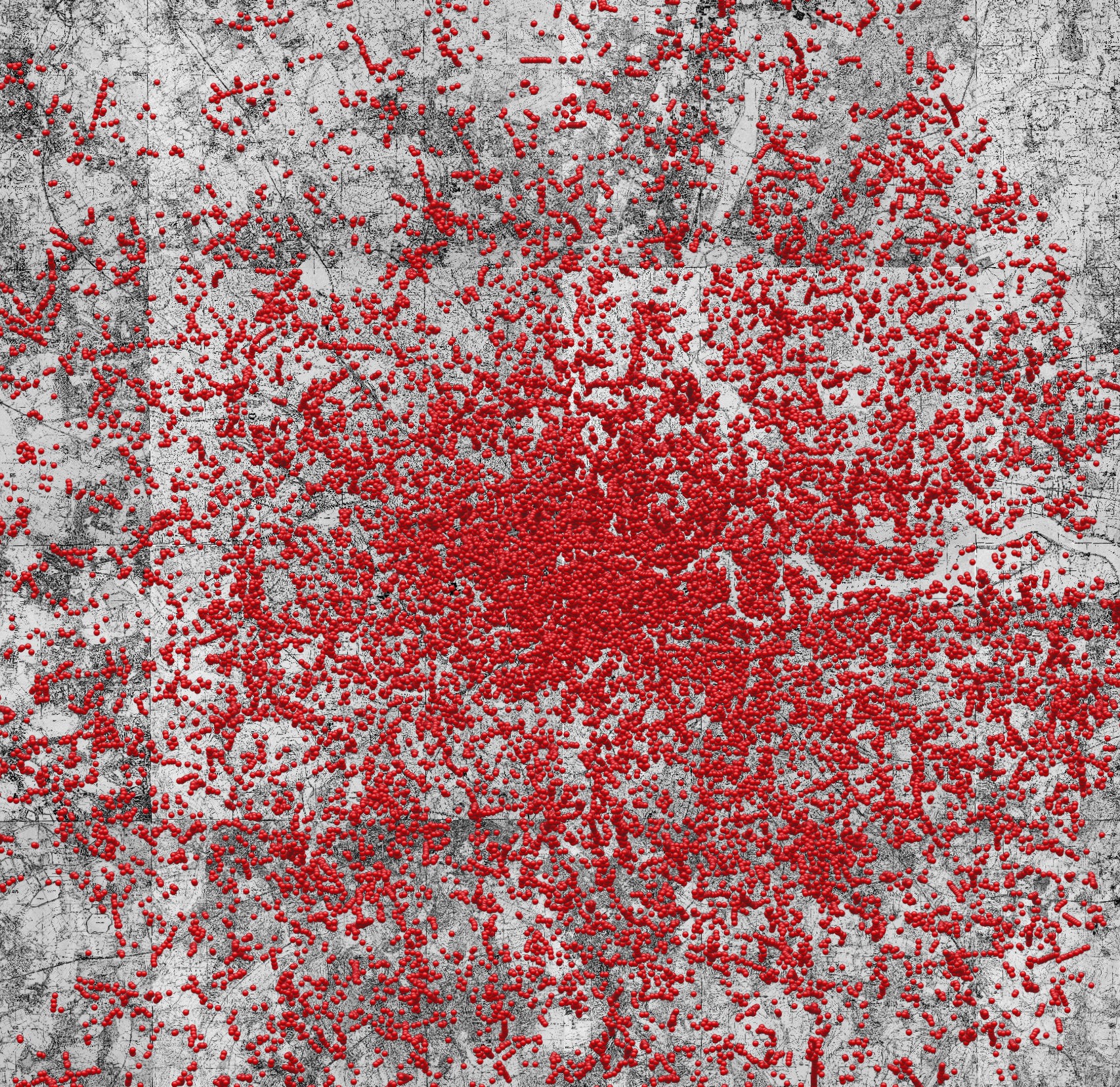
 where, now, F represents the 2-dimensional map and E is used to record both time and location of the bombs. A Poisson point process is a random set of points in E, such that the number that lie within any measurable subset is Poisson distributed. The aim of this post is to introduce Poisson point processes together with the mathematical machinery to handle such random sets.
 are pairwise-disjoint measurable subsets of E, then the sizes of
  are independent.
 -valued stochastic process with independent increments, and which is continuous in probability. Then, the set of points
  over times t for which the jump
  is nonzero gives a Poisson point process on
  . See lemma