Properties of Lévy Processes

Lévy processes, which are defined as having stationary and independent increments, were introduced in the previous post. It was seen that the distribution of a d-dimensional Lévy process X is determined by the characteristics ${(\Sigma,b,\nu)}$ via the Lévy-Khintchine formula,

$\displaystyle \setlength\arraycolsep{2pt} \begin{array}{rl} &\displaystyle{\mathbb E}\left[e^{ia\cdot (X_t-X_0)}\right] = \exp(t\psi(a)),\smallskip\\ &\displaystyle\psi(a)=ia\cdot b-\frac12a^{\rm T}\Sigma a+\int_{{\mathbb R}^d}\left(e^{ia\cdot x}-1-\frac{ia\cdot x}{1+\Vert x\Vert}\right)\,d\nu(x). \end{array}$

(1)

The positive semidefinite matrix ${\Sigma}$ describes the Brownian motion component of X, b is a drift term, and ${\nu}$ is a measure on ${{\mathbb R}^d}$ such that ${\nu(A)}$ is the rate at which jumps ${\Delta X\in A}$ of X occur. Then, equation (1) gives us the characteristic function of the increments of the process.

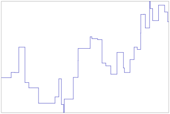
In the current post, I will investigate some of the properties of such processes, and how they are related to the characteristics. In particular, we will be concerned with pathwise properties of X. It is known that Brownian motion and Cauchy processes have infinite variation in every nonempty time interval, whereas other Lévy processes — such as the Poisson process — are piecewise constant, only jumping at a discrete set of times. There are also purely discontinuous Lévy processes which have infinitely many discontinuities, yet are of finite variation, on every interval (e.g., the gamma process).

Let’s start with the simple case of processes with finitely many jumps in each bounded time interval. The proof is given below in the more general case of non-stationary independent increments (see Lemma 6).

Theorem 1 Let X be a cadlag d-dimensional Lévy process with characteristics ${(\Sigma,b,\nu)}$ . Then the following are equivalent.

With positive probability, X has finitely many jumps in some time interval (s,t] with ${s < t}$ .
Almost surely, X has finitely many jumps in every bounded interval.
${\nu(\mathbb{R}^d) < \infty}$ .

Furthermore, if these conditions hold then the number of jumps in the time interval (s,t] has the Poisson distribution with parameter ${(t-s)\nu({\mathbb R}^d)}$ .

For example, this includes homogeneous Poisson processes of rate ${\lambda > 0}$ , where ${X_t-X_s}$ has the Poisson distribution of rate ${\lambda(t-s)}$ . In that case, the Lévy measure is just ${\nu=\lambda\delta_1}$ , where ${\delta_1}$ represents the Dirac measure at 1. More generally, we can construct pure-jump Lévy processes as follows. Fix a constant ${\lambda > 0}$ and probability measure ${\mu}$ on ${{\mathbb R}^d}$ with ${\mu(\{0\})=0}$ . Then, let ${S_1,S_2,\ldots}$ be a sequence of exponentially distributed random variables with parameter ${\lambda}$ and ${Z_1,Z_2,\ldots}$ be ${{\mathbb R}^d}$ -valued variables with measure ${\mu}$ , all of which are independent. Setting ${T_k=\sum_{j=1}^kS_j}$ , then ${N_t\equiv\max\{k\colon S_k\le t\}}$ is a homogeneous Poisson process of rate ${\lambda}$ . We can define the piecewise-constant process

$\displaystyle X_t\equiv\sum_{T_k\le t}Z_k=\sum_{k=1}^{N_t}Z_k,$

which can be seen has stationary independent increments, so it a Lévy process. Then, X is known as a compound Poisson process of rate ${\lambda}$ and jump distribution ${\mu}$ . Its characteristic function can be computed in terms of the characteristic function ${\varphi_\mu(a)\equiv{\mathbb E}[e^{ia\cdot Z_1}]}$ of ${\mu}$ .

$\displaystyle \setlength\arraycolsep{2pt} \begin{array}{rl} \displaystyle{\mathbb E}\left[e^{ia\cdot X_t}\right]&\displaystyle={\mathbb E}\left[{\mathbb E}\left[e^{ia\cdot (Z_1+\cdots+Z_{N_t})}\;\big\vert\; N_t\right]\right]\smallskip\\ &\displaystyle={\mathbb E}\left[\varphi_\mu(a)^{N_t}\right]\smallskip\\ &\displaystyle=\exp\left(\lambda(\varphi_\mu(a)-1)\right) \end{array}$

Substituting in the expression for ${\psi_\mu}$ as an integral with respect to ${\mu}$ gives,

$\displaystyle {\mathbb E}\left[e^{ia\cdot X_t}\right]=\exp\left(\lambda\int_{{\mathbb R}^d}(e^{ia\cdot x}-1)\,d\mu(x)\right)$

Comparing this with the Lévy-Khintchine formula shows that X has Lévy characteristics ${(0,\tilde b,\nu)}$ , where ${\nu=\lambda\mu}$ and

$\displaystyle \tilde b = \int_{{\mathbb R}^d}\frac{x}{1+\Vert x\Vert}\,d\mu(x).$

(2)

Conversely, consider any Lévy process X with characteristics ${(\Sigma,b,\nu)}$ , where ${\nu}$ is finite. By the decomposition into continuous and purely discontinuous parts, we can write this as

$\displaystyle X_t=X_0+W_t+(b-\tilde b)t+Y_t$

where W is a d-dimensional Brownian motion with covariance matrix ${\Sigma}$ , ${\tilde b}$ is given by (2) and Y is a Lévy process with characteristics ${(0,\tilde b,\nu)}$ . Letting ${\lambda=\nu({\mathbb R}^d)}$ and ${\mu}$ be the probability measure ${\lambda^{-1}\nu}$ , we see that Y is a compound Poisson process of rate ${\lambda}$ and jump distribution ${\mu}$ . This, then, describes all Lévy processes whose jumps occur at a finite rate.

Compound Poisson process — Figure 1: A compound Poisson process

We can also give conditions for a Lévy process to have finite variation on bounded intervals. The proof is left until Lemma 7 below.

Theorem 2 Let X be a cadlag d-dimensional Lévy process with characteristics ${(\Sigma,b,\nu)}$ . Then the following are equivalent.

With positive probability, X has finite variation over some time interval (s,t] with ${s < t}$ .
Almost surely, X has finite variation on every bounded interval
${\Sigma=0}$ and

$\displaystyle \int\Vert x\Vert\wedge1\,d\nu(x) < \infty.$

(3)

Furthermore, in this case, we have

$\displaystyle X_t=X_0+(b-\tilde b)t+\sum_{s\le t}\Delta X_s$

(4)

where ${\tilde b}$ is given by (2).

Property (3) is particularly interesting in the case where ${\nu({\mathbb R}^d)}$ is infinite. In that case, X jumps infinitely often but has finite variation in every nonzero bounded time interval. When X is an FV process, it is often convenient to use the decomposition (4), so that we break it up into a constant drift term and a pure jump process Y satisfying ${Y_t=\sum_{s\le t}\Delta Y_s}$ . Such pure jump processes have a particularly simple expression for the characteristic function ${{\mathbb E}[e^{ia\cdot Y_t}]=\exp(t\psi_Y(a))}$ ,

$\displaystyle \psi_Y(a)=\int(e^{ia\cdot x}-1)\,d\nu(x).$

This follows from Theorem 2 by noting that, in this case, ${\tilde b=b}$ so that the Lévy-Khintchine formula simplifies. Comparing with the form of the Lévy-Khintchine formula given in (1), we see that this avoids the rather messy ${ia\cdot x/(1+\Vert x\Vert)}$ term in the integral. However, some purely discontinuous Lévy processes, such as the Cauchy process, do have infinite variation on bounded time intervals, so the more general form in (1) is used.

Real valued and nondecreasing Lévy processes starting from 0 are known as subordinators. In particular, these are finite variation processes, so (3) is satisfied. Subordinators are easily described in terms of their characteristics.

Corollary 3 Let X be a cadlag real valued Lévy process with characteristics ${(0,b,\nu)}$ satisfying (3), and let ${\tilde b}$ be defined by (2).

Then, X is nondecreasing if and only if ${\nu}$ is supported by the positive reals and ${b-\tilde b}$ is nonnegative.

Proof: If X is nondecreasing then its jumps must be nonnegative, so ${\nu({\mathbb R}_-)=0}$ . Also, (4) shows that X has continuous part ${X_t-X_0-\sum_{s\le t}\Delta X_s=(b-\tilde b)t}$ which must be nondecreasing, so ${b-\tilde b\ge0}$ . Conversely, if ${b-\tilde b\ge0}$ and ${\nu({\mathbb R}_-)=0}$ then X has nonnegative jumps and (4) shows that X is nondecreasing. $\Box$

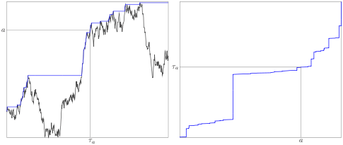
An example of a subordinator can be constructed from hitting times of a standard Brownian motion B started from 0. For each ${a\ge 0}$ , let ${\tau_a}$ be the stopping time

$\displaystyle \tau_a=\inf\left\{t\ge0\colon B_t > a\right\}.$

Considering a as a time index, the process ${a\mapsto\tau_a}$ is right-continuous and increasing. By the strong-Markov property, ${\tilde B_t\equiv B_{\tau_a+t}-a}$ is also a standard Brownian motion independently of ${\tau_a}$ which passes through level b at time ${\tau_{a+b}-\tau_a}$ , so ${\tau_{a+b}-\tau_a\sim\tau_b}$ . From this, we see that ${a\mapsto\tau_a}$ is a subordinator.

At each time ${t\ge0}$ , the Brownian motion B is almost surely strictly less than its maximum ${B^*_t=\sup_{s\le t}B_s}$ , which implies that t is in the union of the intervals ${(\tau_{a-},\tau_a)}$ . So, the union ${\bigcup_{b\le a}(\tau_{b-},\tau_b)}$ almost surely covers almost all of the interval ${[0,\tau_a]}$ . This means that ${\tau_a=\sum_{b\le a}\Delta\tau_a}$ is a pure jump process. We can compute its Lévy measure. We have ${\{\tau_a < u\}=\{B^*_u > a\}}$ and, by the reflection principle, this has probability exactly twice that of ${B_u}$ being greater than a. So, in the limit as a goes to zero,

$\displaystyle \setlength\arraycolsep{2pt} \begin{array}{rl} \displaystyle{\mathbb P}(\tau_a \ge u)&\displaystyle=1-2{\mathbb P}(B_u > a)={\mathbb P}(\vert B_u\vert\le a)\smallskip\\ &\displaystyle=\frac{1}{\sqrt{2\pi}}\int_{-a/\sqrt{u}}^{a/\sqrt{u}}e^{-\frac12x^2}\,dx=a\sqrt{\frac{2}{\pi u}}+o(a). \end{array}$

The Lévy measure of ${\tau}$ satisfies ${\nu([u,\infty))=(2/\pi u)^{1/2}}$ , so ${d\nu(x)=x^{-3/2}dx/\sqrt{2\pi}}$ . Also, using the fact that ${\tilde B_t\equiv u^{-1/2}B_{ut}}$ is a Brownian motion hitting a at time ${u^{-1}\tau_{\sqrt{u}a}}$ , we see that ${\tau_a\sim u^{-1}\tau_{\sqrt{u}a}}$ . In particular, the sum of two independent copies of ${\tau_a}$ has the same distribution as ${\tau_{2a}\sim 4\tau_a}$ . This is equivalent to saying that ${\tau_a}$ is a stable random variable with stability parameter 1/2. Lévy processes whose increments have stable distributions are known as stable processes and, in particular, ${\tau}$ is a stable subordinator. Writing the moment generating function as ${{\mathbb E}[e^{-u\tau_a}]=\exp(-a\varphi(u))}$ , the Lévy-Khintchine formula can be used to calculate ${\varphi(u)=\int(1-e^{-ux})dx/(\sqrt{2\pi} x^{3/2})}$ , from which we obtain ${\varphi(u)=\sqrt{2u}}$ . This verifies the well-known formula for Brownian motion hitting times,

$\displaystyle {\mathbb E}\left[e^{-u\tau_a}\right]=e^{-a\sqrt{2u}}.$

Other examples of subordinators include the gamma process. A gamma process X with mean ${\mu}$ and variance ${\sigma^2}$ per unit time is a Lévy process with ${X_0=0}$ such that ${X_t}$ has the gamma distribution with mean ${\mu t}$ and variance ${\sigma^2t}$ . Setting ${\lambda=\mu/\sigma^2}$ and ${\gamma=\mu^2/\sigma^2}$ , this has probability density function

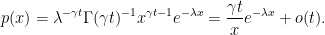$\displaystyle p(x)=\lambda^{-\gamma t}\Gamma(\gamma t)^{-1}x^{\gamma t-1}e^{-\lambda x} =\frac{\gamma t}{x}e^{-\lambda x}+o(t).$

From this, we see that it has Lévy measure ${d\nu(x)=1_{\{x > 0\}}\gamma x^{-1}e^{-\lambda x}\,dx}$ . Furthermore, computing

$\displaystyle {\mathbb E}\left[\sum_{s\le t}\Delta X_s\right]=t\int x\,d\nu(x)=\gamma t/\lambda = {\mathbb E}[X_t]$

we see that the drift term in (4) is zero, so that this is a pure jump process with ${X_t=\sum_{s\le t}\Delta X_s}$ . As it has the gamma distribution, the characteristic function of X is

$\displaystyle {\mathbb E}\left[e^{iaX_t}\right]=\left(1-ia/\lambda\right)^{-\gamma t}.$

Subordinators are often used to apply stochastic time changes to a process. If Z is a Lévy process and, independently, ${t\mapsto\tau_t}$ is a subordinator, then ${X_t\equiv Z_{\tau_t}}$ is another Lévy process. For example, the variance gamma process is a Brownian motion time-changed by a gamma process. Let ${Z_t=B_t+\theta t}$ be a standard Brownian motion with drift ${\theta}$ and ${t\mapsto\tau_t}$ be a gamma process with mean 1 and variance ${\sigma^2}$ per unit time. As ${\tau}$ is a pure jump process, then the variance gamma process is also a pure jump process satisfying ${X_t=\sum_{s\le t}\Delta X_s}$ . Its characteristic function can be calculated from the characteristic functions of the normal and gamma distributions,

$\displaystyle \setlength\arraycolsep{2pt} \begin{array}{rl} \displaystyle{\mathbb E}\left[e^{iaX_t}\right]&\displaystyle={\mathbb E}\left[{\mathbb E}\left[e^{ia(B_{\tau_t}+\theta\tau_t)}\;\big\vert\;\tau_t\right]\right]={\mathbb E}\left[e^{(ia\theta-a^2/2)\tau_t}\right]\smallskip\\ &\displaystyle=\left(1-(ia\theta-a^2/2)/\gamma\right)^{-\gamma t} \end{array}$

where ${\gamma=\sigma^{-2}}$ . Factoring the quadratic into linear terms gives

$\displaystyle \setlength\arraycolsep{2pt} \begin{array}{rl} &\displaystyle {\mathbb E}\left[e^{iaX_t}\right]=\left(1-ia/\lambda_1\right)^{-\gamma t}\left(1+ia/\lambda_2\right)^{-\gamma t}\smallskip\\ &\displaystyle\lambda_1=\sqrt{\theta^2+2\gamma}-\theta,\smallskip\\ &\displaystyle\lambda_2=\sqrt{\theta^2+2\gamma}+\theta. \end{array}$

However, this is just the product of the characteristic function of a gamma process and minus a gamma process, from which we see that variance gamma processes are the difference of independent gamma processes. Therefore, X has Lévy measure

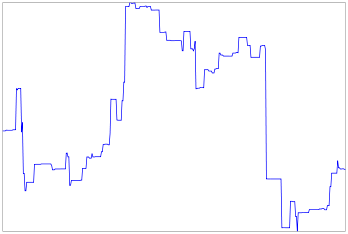
$\displaystyle d\nu(x)=\frac{\gamma}{\vert x\vert}\left(1_{\{x > 0\}}e^{-\lambda_1 x}+1_{\{x < 0\}}e^{-\lambda_2\vert x\vert}\right)\,dx.$

An example of a purely discontinuous Lévy process with infinite variation over all nonzero time intervals is given by the Cauchy process, which is a stable Lévy process with stability parameter ${\alpha=1}$ . If X is a Cauchy process, then ${X_t}$ has the symmetric Cauchy distribution at time t. The probability density function is

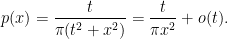$\displaystyle p(x)=\frac{t}{\pi(t^2+x^2)}=\frac{t}{\pi x^2}+o(t).$

So, X has Lévy measure ${d\nu(x)=\pi^{-1}x^{-2}\,dx}$ . In particular, as ${\int_{-1}^1\vert x\vert\,d\nu(x)=\infty}$ , inequality (3) does not hold and, consequently, X is not a finite variation process.

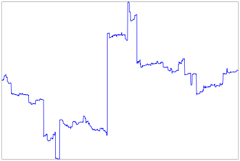
It is possible to determine the integrability of a Lévy process from its Lévy measure. In fact, integrability is equivalent to the apparently much weaker property of local integrability, and is also equivalent to the seemingly much stronger condition of integrability of its maximum process. The proof of the following theorem will be given in Lemma 8 below for the more general situation of inhomogeneous independent increments processes.

Theorem 4 Let X be a cadlag d-dimensional Lévy process with ${X_0=0}$ and let p be a real number in ${[1,\infty)}$ . Then, the following are equivalent.

X is locally ${L^p}$ -integrable.
X is ${L^p}$ -integrable.
${X^*_t\equiv\sup_{s\le t}\Vert X_s\Vert}$ is ${L^p}$ -integrable.
The Lévy measure ${\nu}$ satisfies ${\int_{\Vert x\Vert\ge1} \Vert x\Vert^p\,d\nu(x) < \infty}$ .

So each of the examples of Lévy processes mentioned above are integrable, with the exceptions of the 1/2-stable process of Brownian hitting times and the Cauchy process.

Note that if X is an integrable Lévy process then ${X-{\mathbb E}[X]}$ has independent increments of mean zero, so is a martingale. It is therefore possible, and often convenient, to decompose such processes as the sum of a constant drift term and a martingale Lévy process.

Lemma 5 Let X be an ${L^p}$ -integrable Lévy process with characteristics ${(\Sigma,b,\nu)}$ . Then it uniquely decomposes as

$\displaystyle X_t=X_0+b^{\prime}t+W_t+M_t$

(5)

where ${b^\prime\in{\mathbb R}^d}$ , W is a Brownian motion with covariance matrix ${\Sigma}$ and M is an ${L^p}$ -integrable martingale with characteristic function ${{\mathbb E}[e^{ia\cdot M_t}]=\exp(t\psi_M(a))}$ where,

$\displaystyle \psi_M(a)=\int\left(e^{ia\cdot x}-1-ia\cdot x\right)\,d\nu(x).$

(6)

As ${\vert e^{ia\cdot x}-1-ia\cdot x\vert\le\vert a\cdot x\vert + 2}$ , the final statement of Theorem 4 implies that the integral in (6) is well-defined. The proof of this Lemma follows quickly from previous results of these notes. First, for any ${b^\prime\in{\mathbb R}^d}$ , decomposition (5) follows from the decomposition of X into its purely continuous and discontinuous parts, W and M respectively. Then, M is an ${L^p}$ -integrable Lévy process with characteristics ${(0,b-b^\prime,\nu)}$ . Setting

$\displaystyle b^\prime = b + \int\left(x-\frac{x}{1+\Vert x\Vert}\right)\,d\nu(x)$

then (6) follows from the Lévy-Khintchine formula. It only remains to show that M is a martingale and, by the independent increments property, it is enough to show that it has zero mean. Using dominated convergence to commute the differentiation with the integral in (6), we can calculate

$\displaystyle \nabla\psi_M(a)=i\int\left(e^{ia\cdot x}-1\right)x\,d\nu(x).$

So, differentiating (6) at a=0 gives ${{\mathbb E}[M_t]=t\nabla\psi_M(0)=0}$ .

Inhomogeneous independent increments processes

All of the results given above apply equally to time-inhomogeneous independent increments processes, and I will now go through their proofs at this level of generality. Throughout this section, it is assumed that X is a cadlag d-dimensional process with independent increments, and which is continuous in probability. As previously shown, the increments of such a process have characteristic function of the form

$\displaystyle \setlength\arraycolsep{2pt} \begin{array}{c} \displaystyle{\mathbb E}\left[e^{ia\cdot(X_t-X_0)}\right]=e^{i\psi_t(a)},\smallskip\\ \displaystyle\psi_t(a)=ia\cdot\tilde b_t-\frac12a^{\rm T}\tilde\Sigma_ta+\int_{[0,t]\times{\mathbb R}^d}\left(1-e^{ia\cdot x}-\frac{ia\cdot x}{1+\Vert x\Vert}\right)\,d\mu(s,x). \end{array}$

(7)

Here, ${\tilde\Sigma\colon{\mathbb R}_+\rightarrow{\mathbb R}^{d\times d}}$ is a map from time t to a symmetric ${d\times d}$ matrix ${\tilde\Sigma_t}$ with ${\tilde\Sigma_0=0}$ and is increasing in the sense that ${\tilde\Sigma_t-\tilde\Sigma_s}$ is positive semidefinite for all ${t\ge s}$ . Also, ${\tilde b\colon{\mathbb R}_+\rightarrow{\mathbb R}^d}$ is a continuous function starting from zero, and ${\mu}$ is a Borel measure on ${{\mathbb R}_+\times{\mathbb R}^d}$ such that ${\mu({\mathbb R}_+\times\{0\})=\mu(\{t\}\times{\mathbb R}^d)=0}$ for all ${t\ge0}$ , and

$\displaystyle \int_{[0,t]\times{\mathbb R}^d}\Vert x\Vert^2\wedge1\,d\mu(s,x) < \infty.$

In the case where X also has stationary increments, so that it is a Lévy process, then ${(\tilde\Sigma,\tilde b,\mu)}$ are related to the Lévy characteristics ${(\Sigma,b,\nu)}$ by ${\tilde\Sigma_t=t\Sigma}$ , ${\tilde b=tb}$ and ${d\mu(t,x)=dt\,d\nu(x)}$ . In that case, equation (7) reduces to the standard Lévy-Khintchine formula.

We start by giving a proof of Theorem 1 which, just being a re-statement of results previously covered in these note, is particularly simple.

Lemma 6 The following are equivalent.

With positive probability, X has finitely many jumps.
With probability one, X has finitely many jumps.
${\mu({\mathbb R}_+\times{\mathbb R}^d)}$ is finite.

In this case, the number of jumps of X is Poisson distributed with rate ${\mu({\mathbb R}_+\times{\mathbb R}^d)}$ .

Proof: Letting ${\eta}$ be the total number of jumps of ${X}$ , then this is just a restatement of the fact that ${\eta}$ is Poisson distributed with rate ${\lambda=\mu({\mathbb R}_+\times{\mathbb R}^d)}$ whenever ${\lambda}$ is finite, and ${\eta}$ is almost surely infinite whenever ${\lambda}$ is infinite. $\Box$

Theorem 1 is an immediate consequence of this. If X is a Lévy process with characteristics ${(\Sigma,b,\nu)}$ , then the first statement of Theorem 1 implies that there is a non-trivial time interval [s,t] on which, with positive probability, X has finitely many jumps. Applying Lemma 6 to X restricted to this interval implies that ${\mu([s,t]\times{\mathbb R}^d)=(t-s)\nu({\mathbb R}^d)}$ is finite. So, ${\nu({\mathbb R}^d) <\infty}$ and it follows that ${\mu([s,t]\times{\mathbb R}^d)}$ is finite for all ${s < t}$ and, again applying Lemma 6, the number of jumps in any finite time interval [s,t] is almost surely finite with the Poisson distribution of rate ${(t-s)\nu({\mathbb R}^d)}$ .

I now give a proof of the following generalization of Theorem 2.

Lemma 7 Let ${f\colon{\mathbb R}_+\times{\mathbb R}^d\rightarrow{\mathbb R}}$ be a measurable function satisfying ${f(t,0)=0}$ , and set ${V=\sum_{t > 0}\vert f(t,\Delta X_t)\vert}$ . The following are equivalent,

With positive probability, V is finite.
With probability one, V is finite.
${\mu(\vert f\vert\wedge1) < \infty}$ .

In this case, setting ${U=\sum_{t > 0}f(t,\Delta X_t)}$ , then

$\displaystyle {\mathbb E}\left[e^{iaU}\right]=\exp\left(\mu(e^{iaf}-1)\right).$

(8)

for all real a.

Proof: This result actually holds in the generality of Poisson point processes although, here, we are only concerned with the application to independent increments processes. Let us start by considering the case where ${\mu(\vert f\vert\wedge1)}$ is finite. In that case, the identity

$\displaystyle {\mathbb E}\left[\sum_{t>0}\vert f(t,\Delta X_t)\vert\wedge1\right]=\mu(\vert f\vert\wedge1)$

shows that V is almost-surely finite. So, ${Y_t\equiv\sum_{s\le t}f(s,\Delta X_s)}$ is a well-defined independent increments process. Therefore, its characteristic function is of the form ${{\mathbb E}[e^{iaY_t}]=\exp(\tilde\psi_t(a))}$ where

$\displaystyle \setlength\arraycolsep{2pt} \begin{array}{rl} \displaystyle M_t&\displaystyle\equiv iaY_t-\tilde\psi_t(a)-\frac12a^2[Y]^c_t-\sum_{s\le t}\left(e^{ia\Delta Y_s}-1-ia\Delta Y_s\right)\smallskip\\ &\displaystyle=-\tilde\psi_t(a)-\sum_{s\le t}\left(e^{iaf(s,\Delta X_s)}-1\right) \end{array}$

is a square integrable martingale. Taking expectations and letting t increase to infinity, so that ${Y_t\rightarrow U}$ , gives

$\displaystyle \setlength\arraycolsep{2pt} \begin{array}{rl} \displaystyle{\mathbb E}\left[e^{iaU}\right]&\displaystyle=\exp\left({\mathbb E}\left[\sum_{s\ge0}\left(e^{iaf(s,\Delta X_s)}-1\right)\right]\right)\smallskip\\ &\displaystyle=\exp\left(\mu\left(e^{iaf}-1\right)\right) \end{array}$

as required. Note that the inequality ${\vert e^{iaf}-1\vert\le \vert af\vert\wedge2}$ implies that ${e^{iaf}-1}$ is ${\mu}$ -integrable, so this expression is always well defined.

It only remains to show that all this holds whenever V is finite with nonzero probability. Consider, for the moment, the case where ${f}$ is nonnegative and ${\mu(f\wedge1) < \infty}$ . Then, ${e^{iaf}}$ is uniformly bounded for all complex a with nonnegative imaginary part and, by analytic continuation (8) extends to all such a. So, we can replace a by ia to get

$\displaystyle {\mathbb E}\left[e^{-aU}\right]=\exp\left(-\mu\left(1-e^{-af}\right)\right).$

(9)

for all ${a > 0}$ . However, this identity extends to all nonnegative f. Simply apply it to a sequence of nonnegative functions ${f_n\uparrow f}$ with ${\mu(f_n\wedge1) < \infty}$ and use dominated convergence on the left and monotone convergence on the right to take the limit as n goes to infinity. Suppose that the third property of the statement of the Lemma did not hold, so that ${\mu(f\wedge1)=\infty}$ . Then, the inequality ${1-e^{-af}\ge\frac12((af)\wedge1)}$ gives ${\mu(1-e^{-af})=\infty}$ for all positive a. So, the right hand side of (9) is zero. Taking the limit as a decreases to 0,

$\displaystyle {\mathbb P}(U<\infty)=\lim_{a\rightarrow0}{\mathbb E}\left[e^{-aU}\right]=0.$

Conversely, if ${U\equiv\sum_{t>0}f(t,\Delta X_t)}$ has nonzero probability of being finite, then we see that ${\mu(f\wedge1)}$ must be finite. Applying this to ${\vert f\vert}$ for arbitrary (not necessarily positive) f shows that the first condition of the Lemma implies the third. $\Box$

To show that this result implies Theorem 2, consider a Lévy process X with characteristics ${(\Sigma,b,\mu)}$ . As the continuous part of its quadratic variation, ${[X]^c_t=t\Sigma}$ is constant over any interval on which X has finite variation, the first condition of Theorem 2 implies that ${\Sigma}$ is zero. If X has finite variation with positive probability over an interval [s,t], Lemma 7 applied to ${V\equiv\sum_{s < u\le t}\Vert\Delta X_u\Vert}$ shows that

$\displaystyle \int_{[s,t]\times{\mathbb R}^d}\Vert x\Vert\wedge1\,d\mu(u,x)=(t-s)\nu(\Vert x\Vert\wedge1)$

is finite. So, ${\nu(\Vert x\Vert\wedge1) < \infty}$ . Then, applying the lemma to any interval [0,t] shows that ${\sum_{s\le t}\Vert \Delta X_s\Vert}$ is almost surely finite, so ${Z_t\equiv X_t-\sum_{s\le t}\Delta X_s}$ is well defined. As this is a continuous Lévy process with zero quadratic variation, it is simply of the form ${Z_t=X_0+ct}$ for a constant ${c\in{\mathbb R}^d}$ . So, X almost surely has finite variation over all bounded time intervals. To calculate c, we can apply (8) with ${f(t,x)=ia\cdot x}$ to obtain

$\displaystyle \setlength\arraycolsep{2pt} \begin{array}{rl} \displaystyle{\mathbb E}\left[e^{ia\cdot(X_t-X_0)}\right]&\displaystyle={\mathbb E}\left[e^{ia\cdot c+\sum_{s\le t}ia\cdot\Delta X_s}\right]\smallskip\\ &\displaystyle=\exp\left(ia\cdot ct+\int_{[0,t]\times{\mathbb R}^d}(e^{ia\cdot x}-1)\,d\mu(s,x)\right)\smallskip\\ &\displaystyle=\exp\left(ia\cdot ct+t\int(e^{iax}-1)\,d\nu(x)\right) \end{array}$

Comparing this with the Lévy-Khintchine formula (1) gives ${c=b-\tilde b}$ with ${\tilde b}$ as in equation (2). So (4) holds, and Theorem 2 follows.

Finally, we give a proof of Theorem 4 for independent increments processes.

Lemma 8 Suppose that ${X_0=0}$ and choose any ${1\le p < \infty}$ . Then, the following are equivalent.

X is locally ${L^p}$ -integrable.
X is ${L^p}$ -integrable.
${X^*_t\equiv\sup_{s\le t}\Vert X_s\Vert}$ is ${L^p}$ -integrable.
For all times ${t\ge0}$

$\displaystyle \int_{[0,t]\times{\mathbb R}^d}1_{\{\Vert x\Vert\ge1\}}\Vert x\Vert^p\,d\mu(s,x) < \infty.$

(10)

Proof: First, consider any nonnegative measurable function ${f\colon{\mathbb R}^d\rightarrow{\mathbb R}}$ such that

$\displaystyle c_t\equiv\int_{[0,t]\times{\mathbb R}^d}f(x)\,d\mu(s,x)$

is finite for all ${t\ge0}$ . Then, taking ${Y_t=\sum_{s\le t}1_{\{\Delta X_s\not=0\}}f(\Delta X_s)}$ , we know that ${Y-c}$ is a martingale so, by optional stopping,

$\displaystyle {\mathbb E}[Y_{t\wedge\tau}]={\mathbb E}[c_{t\wedge\tau}]\ge c_t{\mathbb P}(\tau\ge t)$

(11)

for all stopping times ${\tau}$ . Note that this extends to all nonnegative measurable ${f}$ . Just apply it to a sequence ${0\le f_n\le f}$ increasing to ${f}$ such that ${\int_{[0,t]\times{\mathbb R}^d}f_n(x)\,d\mu(s,x)}$ is finite, and use monotone convergence as n goes to infinity. In particular, consider ${f(x)=1_{\{\Vert x\Vert\ge1\}}\Vert x\Vert^p}$ . In that case ${\Delta Y\le\Vert\Delta X\Vert^p}$ . If property 1 holds so that X is locally ${L^p}$ -integrable, then Y is locally integrable. Therefore, there is a stopping time ${\tau}$ with ${{\mathbb P}(\tau\ge t) > 0}$ and ${{\mathbb E}[Y_\tau] < \infty}$ . Applying (11) to this gives

$\displaystyle c_t{\mathbb P}(\tau\ge t)\le{\mathbb E}[Y_{\tau}] < \infty.$

So ${c_t}$ is finite and (10) holds.

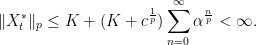
Conversely, supposing that (10) holds, it only remains to be shown that ${X^*_t}$ is ${L^p}$ -integrable for each fixed time t. To do this, fix a constant ${K > 0}$ and define stopping times ${\tau_0=0}$ and

$\displaystyle \tau_{n+1}=\inf\left\{s\ge\tau_n\colon\Vert X_s-X_{\tau_n}\Vert\ge K\right\}$

for ${n\ge0}$ . For each time ${s\le t}$ , there almost surely exists an n with ${\tau_n \le s < \tau_{n+1}}$ , so ${\Vert X_s-X_{\tau_n}\Vert < K}$ . Therefore, we can bound ${X^*_t}$ in the ${L^p}$ norm by

$\displaystyle \Vert X^*_t\Vert_p\le K+\sum_{n=0}^\infty\Vert X_{\tau_{n+1}\wedge t}-X_{\tau_n\wedge t}\Vert_p.$

(12)

Noting that ${X_{\tau_{n+1}\wedge t}-X_{\tau_n\wedge t}}$ is bounded by ${K+\Vert\Delta X_{\tau_{n+1}\wedge t}\Vert}$ whenever ${\tau_n < t}$ and zero otherwise, its ${L^p}$ norm satisfies the bound

$\displaystyle \Vert X_{\tau_{n+1}\wedge t}-X_{\tau_n\wedge t}\Vert_p\le K\Vert 1_{\{\tau_n < t\}}\Vert_p+\left\Vert 1_{\{\tau_n < t\}}\Delta X_{\tau_{n+1}\wedge t}\right\Vert_p.$

(13)

The terms on the right hand side can be bounded as follows. By the independent increments property, for all times ${s < t}$ ,

$\displaystyle \setlength\arraycolsep{2pt} \begin{array}{rl} \displaystyle{\mathbb P}\left(\sup_{u\in(s,t]}\Vert X_u-X_s\Vert\ge K\;\middle\vert\;\mathcal{F}_s\right)&\displaystyle={\mathbb P}\left(\sup_{u\in(s,t]}\Vert X_u-X_s\Vert\ge K\right)\smallskip\\ &\displaystyle\le{\mathbb P}\left(\sup_{u,v\le t}\Vert X_u-X_v\Vert\ge K\right). \end{array}$

Using ${\alpha}$ to denote the term on the right hand side, we can assume that K has been chosen large enough that this is strictly less than 1 (actually, this is true for all positive K). Then, as the space-time process ${(s,X_s)}$ is a Feller process and, hence, satisfies the strong Markov property, this inequality holds when s is replaced by a stopping time. Replacing s by ${\tau_n\wedge t}$ gives ${{\mathbb P}(\tau_{n+1}\le t\mid\mathcal{F}_{\tau_n})\le\alpha}$ . So, ${{\mathbb P}(\tau_{n+1} < t)\le\alpha{\mathbb P}(\tau_n < t)}$ and, by induction, we see that ${{\mathbb P}(\tau_n < t)}$ is bounded by ${\alpha^n}$ .

Again using the independent increments property for ${s < t}$ ,

$\displaystyle \setlength\arraycolsep{2pt} \begin{array}{rl} \displaystyle{\mathbb E}\left[\sup_{u\in(s,t]}\Vert\Delta X_u\Vert^p\;\middle\vert\;\mathcal{F}_s\right]&\displaystyle={\mathbb E}\left[\sup_{u\in(s,t]}\Vert\Delta X_u\Vert^p\right]\smallskip\\ &\displaystyle\le1+{\mathbb E}\left[\sum_{u\le t}1_{\{\Vert\Delta X_u\Vert\ge1\}}\Vert\Delta X_u\Vert^p\right]\smallskip\\ &\displaystyle=1+\int_{[0,t]\times{\mathbb R}^d}1_{\{\Vert x\Vert\ge1\}}\Vert x\Vert^p\,d\mu(u,x). \end{array}$

Denote the right hand side by c which, by (10), is finite. Applying the strong Markov property again to replace s by ${\tau_n\wedge t}$ , this gives

$\displaystyle \setlength\arraycolsep{2pt} \begin{array}{rl} \displaystyle{\mathbb E}\left[1_{\{\tau_n < t\}}\Vert\Delta X_{\tau_{n+1}\wedge t}\Vert^p\right]&\displaystyle={\mathbb E}\left[1_{\{\tau_n < t\}}{\mathbb E}\left[\Vert\Delta X_{\tau_{n+1}\wedge t}\Vert^p\;\middle\vert\;\mathcal{F}_{\tau_n}\right]\right]\smallskip\\ &\displaystyle\le c{\mathbb P}(\tau_n < t)\le c\alpha^n. \end{array}$

Putting these bounds back into (13),

$\displaystyle \Vert X_{\tau_{n+1}\wedge t}-X_{\tau_n\wedge t}\Vert_p\le (K+c^{\frac1p})\alpha^{\frac{n}{p}}.$

Finally putting this back into (12) gives the required bound

$\displaystyle \Vert X_t^*\Vert_p\le K+(K+c^{\frac1p})\sum_{n=0}^\infty\alpha^{\frac{n}{p}} < \infty.$

$\Box$

14 thoughts on “Properties of Lévy Processes”

Rob says:

10 March 11 at 5:05 AM

George,

I’ve been working my way into the stochastic processes space and was wondering if you could recommend any good books/papers on Levy processes. Your write ups on Levy processes and all things stochastic are top notch, but I was hoping to get a deeper understanding of the field. Any help would be appreciated.

Thanks.

PS Keep up the quality work. It’s certainly been a good read so far.

1. George Lowther says:
  
  11 March 11 at 1:41 AM
  
  Hi.
  
  I’m not sure what to recommend. My knowledge is really drawn from a wide variety of sources over a long period of time, but nothing specifically dedicated to Lévy processes. On hand I have Protter, which is a great book, but mainly for general stochastic calculus with only a short section on Lévy processes, Kallenberg, which goes into a bit more depth but still only one chapter, and He, Wang & Yan which is very rigorous and a great reference but, again, mainly for general stochastic processes.
  
  On the other hand, there are books concentrating on Lévy processes and many concentrating on specific areas of application (particularly, in Finance). But I’m not sure which of these to recommend. Sorry I can’t be of more help here.
  
  1. Rob says:
    
    12 March 11 at 1:07 AM
    
    Thanks. I’ll definitely look into those. The fact that they aren’t “Levy specific” is no big deal. I’ve been in need of some stochastic calculus references. Your help is certainly appreciated.
    
    Rob
    
    1. Zhenyu (Rocky) Cui says:
      
      11 April 11 at 2:19 PM
      
      For general Levy process theory, I recommend the book “Lévy process and infinitely divisible distributions” by Ken Iti Sato. The Amazon link is: http://www.amazon.com/Processes-Infinitely-Divisible-Distributions-Mathematics/dp/0521553024
      
      For more modern account of Levy process, like fluctuation theory and new examples of scale functions, etc, I recommend the book: “ Introductory Lectures on Fluctuations of Lévy Processes with Applications” at: http://www.amazon.com/Introductory-Fluctuations-Processes-Applications-Universitext/dp/3540313427/ref=pd_sim_b_4
      
      Hope this helps and Bon Appetit~ 🙂
Rob says:

11 April 11 at 5:05 PM

Rocky,

Thanks for the recommendations. I’ll be sure to add those to my “summer reading list” … assuming I’m not too burnt out from my upcoming qualifier.

Rob

1. Zhenyu (Rocky) Cui says:
  
  12 April 11 at 3:12 AM
  
  Hello, Rob,
  
  I just passed my Ph.D comprehensive exams and I understand the efforts and pain taken~ If you want a working knowledge of Levy process and are interested mostly in applications such as finance, then Cont and Tankov’s book is more user friendly and explains many heuristic ideas behind Levy process. Check it out: http://www.amazon.com/Financial-Modelling-Processes-Chapman-Mathematics/dp/1584884134
  
  Rocky 🙂
  
Steve says:

5 October 11 at 11:45 AM

Hi George,
can you please clarify the proof of Brownian hitting times being a subordinator? I feel I’m missing something on the understanding of the argument given here!
Thank you very much, keep up the great work!

Steve

1. George Lowther says:
  
  5 October 11 at 10:38 PM
  
  Hi. The point is that (i) The difference of stopping times $\tau_{a+b}-\tau_a$ is just the first time that $\hat B_t\equiv B_{\tau_a+t}-B_{\tau_a}$ hits $b$ . (ii) The strong Markov property says that $\hat B$ is a Brownian motion independent of $\mathcal{F}_{\tau_a}$ . So, (iii) $\tau_{a+b}-\tau_a$ has the same distribution as $\tau_a$ and (iv) $\tau_{a+b}-\tau_a$ is independents of $\tau_a$ . Therefore $a\mapsto\tau_a$ has independent and identically distributed increments. To say that it is a subordinator, you just need to show that it is right-continuous and non-decreasing. But (v) that it is increasing is immediate from the definition and (vi) right-continuity follows from the continuity of Brownian paths. So $a\mapsto\tau_a$ is a subordinator.
  
  Did you follow that? Or was one of the points (i)-(vi) unclear?
  
  1. Steve says:
    
    7 October 11 at 1:58 PM
    
    Ok, now it’s perfectly clear, I follow that.
    thank you very much for your prompt response!
    
    Great blog by the way, keep up the good work!
    
    Steve
    
Andrea says:

8 June 12 at 3:29 PM

Hi George,
can you please specify why a subordinated Levy process via an independent subordinator is still a Levy process?
Thank you very much, your blog is fantastic!

1. George Lowther says:
  
  13 July 12 at 12:37 AM
  
  If X is a Lévy process and τ is an independent subordinator, then you need to show that X_τ has independent identically distributed increments. For any finite increasing sequence of times $t_1\le t_1\le\cdots\le t_n$ and bounded measurable functions $f_k\colon\mathbb{R}^d\to\mathbb{R}$ , you have the following sequence of equalities.
  
  $\setlength\arraycolsep{2pt}\begin{array}{rl} \displaystyle \mathbb{E}\left[\prod_kf_k(X_{\tau_{t_k}}-X_{\tau_{t_{k-1}}})\right]&\displaystyle=\mathbb{E}\left[\mathbb{E}\left[\prod_kf_k(X_{\tau_{t_k}}-X_{\tau_{t_{k-1}}})\;\vert\tau_\cdot\right]\right]\smallskip\\ &\displaystyle=\mathbb{E}\left[\prod_k\mathbb{E}\left[f_k(X_{\tau_{t_k}}-X_{\tau_{t_{k-1}}})\;\vert\tau_\cdot\right]\right]\smallskip\\ &\displaystyle=\mathbb{E}\left[\prod_k\mathbb{E}\left[f_k(X_{\tau_{t_k}-\tau_{t_{k-1}}}-X_{\tau_0})\;\vert\tau_\cdot\right]\right]\smallskip\\ &\displaystyle=\prod_k\mathbb{E}\left[\mathbb{E}\left[f_k(X_{\tau_{t_k}-\tau_{t_{k-1}}}-X_{\tau_0})\;\vert\tau_{t_k}-\tau_{t_{k-1}}\right]\right]\smallskip\\ &\displaystyle=\prod_k\mathbb{E}\left[f_k(X_{\tau_{t_k}}-X_{\tau_{t_{k-1}}})\right]\smallskip\\ &\displaystyle=\prod_k\mathbb{E}\left[f_k(X_{\tau_{t_k-t_{k-1}}}-X_0)\right] \end{array}$
  
  First, the expectation is conditioned on τ. The second equality is just independence of increments for X. The third is indentical increments for X. The fourth is independent increments for τ, and the sixth is identical increments for τ. Applying this equality for n = 1 gives identical increments for X_τ. Then, applying this for n ≥ 1 and noting that the right hand side is just the product of the expectations gives independence. (Apologies for the slow response to your comment).
  
Michael K. says:

14 April 16 at 10:11 AM

Thank you for this wonderful and useful webpage. I have a question about alpha stable processes. If L is such a process, what is the quadratic variation of dL i.e. [dL] = [dL,dL]?

1. George Lowther says:
  
  6 June 16 at 12:54 AM
  
  Well, if L is alpha-stable, then you can show that [L] will be an increasing alpha/2-stable process.
  
Jaehun Lee says:

25 January 18 at 5:26 AM

Could you let me know the reference for Theorem 4?

	Tavin on Class (D) Processes
	George Lowther on Filtrations and Adapted P…
	faceet on Filtrations and Adapted P…
	George Lowther on Filtrations and Adapted P…
	facet on Filtrations and Adapted P…
	Zoltan on Class (D) Processes
	Zoltan on Class (D) Processes
	ARS on Stopping Times and the Debut…
	George Lowther on Upcrossings, Downcrossings, an…
	George Lowther on Stopping Times and the Debut…

Properties of Lévy Processes

Published by George Lowther

14 thoughts on “Properties of Lévy Processes”

Leave a Reply Cancel reply

Like this:

Related

Published by George Lowther

14 thoughts on “Properties of Lévy Processes”

Leave a Reply Cancel reply