Local Time Continuity

Local time surface — Figure 1: Brownian motion and its local time surface

The local time of a semimartingale at a level x is a continuous increasing process, giving a measure of the amount of time that the process spends at the given level. As the definition involves stochastic integrals, it was only defined up to probability one. This can cause issues if we want to simultaneously consider local times at all levels. As x can be any real number, it can take uncountably many values and, as a union of uncountably many zero probability sets can have positive measure or, even, be unmeasurable, this is not sufficient to determine the entire local time ‘surface’

$\displaystyle (t,x)\mapsto L^x_t(\omega)$

for almost all ${\omega\in\Omega}$ . This is the common issue of choosing good versions of processes. In this case, we already have a continuous version in the time index but, as yet, have not constructed a good version jointly in the time and level. This issue arose in the post on the Ito–Tanaka–Meyer formula, for which we needed to choose a version which is jointly measurable. Although that was sufficient there, joint measurability is still not enough to uniquely determine the full set of local times, up to probability one. The ideal situation is when a version exists which is jointly continuous in both time and level, in which case we should work with this choice. This is always possible for continuous local martingales.

Theorem 1 Let X be a continuous local martingale. Then, the local times

$\displaystyle (t,x)\mapsto L^x_t$

have a modification which is jointly continuous in x and t. Furthermore, this is almost surely ${\gamma}$ -Hölder continuous w.r.t. x, for all ${\gamma < 1/2}$ and over all bounded regions for t.

A proof will be given further down. Theorem 1 applies, in particular, to Brownian motion although, in this case, the continuous modification also satisfies the stronger property of joint Hölder continuity.

Theorem 2 Let X be a Brownian motion with arbitrary starting value. Then, the jointly continuous version of the local times ${L^x_t}$ are almost surely jointly ${\gamma}$ -Hölder continuous in x and t, for all ${\gamma < 1/2}$ and bounded intervals for t.

Again, the proof will be given further down. In fact, theorem 2 can be used to determine the joint continuity properties for the local times of any continuous local martingale, giving an improvement over the previous result. We know that any local martingale X can be written as a time-change of a standard Brownian motion B started from ${X_0}$ . Specifically, ${X_t=B_{[X]_t}}$ , where ${[X]}$ is the quadratic variation. Also, local times transform in the expected way under continuous time changes. If we write ${\tilde L^x_t}$ for the local times of B which, by theorem 2, is locally Hölder continuous in x and t, then the local time of X is

$\displaystyle L^x_t=\tilde L^x_{[X]_t}.$

This shows that ${L^x_t}$ has a version which is a locally ${\gamma}$ -Hölder continuous function of ${[X]_t}$ and x for all ${\gamma < 1/2}$ .

Next, consider more general continuous semimartingales. It turns out that, now, the local times need not have a jointly continuous version. For example, if B is a Brownian motion, then ${X=\lvert B\rvert}$ is a reflected Brownian motion. Writing ${\tilde L^x_t}$ for the local times of B, then the local times of X are given by,

$\displaystyle L^x_t=1_{\{x\ge0\}}\left(\tilde L^x_t+\tilde L^{-x}_t\right).$

This is jointly continuous when x is away from 0 but, as x passes through 0, then ${L^x_t}$ jumps by twice the local time of B. The best that we can hope for is that ${L^x_t}$ is jointly continuous in t and cadlag in x. This means that for each ${(t,x)\in{\mathbb R}_+\times{\mathbb R}}$ then there exists a left-limit ${L^{x-}_t=\lim_{y\uparrow\uparrow x}L^y_t}$ such that, for sequences ${t_n\rightarrow t}$ and ${x_n\rightarrow x}$ ,

$\displaystyle L^{x_n}_{t_n}\rightarrow\begin{cases} L^x_t,&{\rm if\ }x_n\ge x{\rm\ for\ all\ }n,\\ L^{x-}_t&{\rm if\ }x_n < x{\rm\ for\ all\ }n. \end{cases}$

Equivalently, considered as a set of continuous functions ${t\mapsto L^x_t}$ , one for each x, then ${x\mapsto L^x}$ is cadlag under the topology of uniform convergence on compacts.

Theorem 3 Let X be a continuous semimartingale. Then, its local times ${L^x_t}$ have a version which is jointly continuous in t and cadlag in x.

Furthermore, if ${X=M+V}$ is the decomposition into a continuous local martingale and FV process V then, with probability one,

$\displaystyle L^x_t-L^{x-}_t = 2\int_0^t1_{\{X=x\}}dV$

for all times t and levels x.

We can further ask whether the semimartingale X needs to be continuous in order that the local times have a modification as in the theorem above. In fact, it is possible to extend to a class of non-continuous processes but, unfortunately, not to all semimartingales. This will be stated in a moment, and theorem 3 will follow from this more general result. We need to restrict to a class of semimartingales whict have only a finite variation coming from the jumps, which can be expressed in a couple of different ways.

Lemma 4 Let X be a semimartingale. Then, the following are equivalent,

${\sum_{s\le t}\lvert\Delta X_s\rvert < \infty}$ , almost surely for all times t.

X decomposes as the sum of a continuous local martingale and an FV process.

Furthermore, in this case, X decomposes as

$\displaystyle X_t = M_t + V_t + \sum_{s\le t}\Delta X_s$ (1)

for a continuous local martingale M and continuous FV process V.

Proof: If the first condition holds, then we can define the pure jump process ${J_t=\sum_{s\le t}\Delta X_s}$ . So, ${X-J}$ is a continuous semimartingale and, therefore, decomposes into the sum of a continuous local martingale M and continuous FV process V. This gives decomposition (1) and, as ${V+J}$ is an FV process, also implies the second condition.

Conversely, if the second condition holds, then write ${X=M+V}$ for continuous local martingale M and FV process V. As ${\Delta X=\Delta V}$ , the sum ${\sum_{s\le t}\lvert\Delta X_s\rvert}$ is equal to ${\sum_{s\le t}\lvert\Delta V_s\rvert}$ . As this is bounded by the variation of V, it is almost surely finite. ⬜

We will restrict to the class of processes identified by the equivalent conditions above. I am not aware of any standard terminology for referring to such semimartingales other than the following definition as used by Protter, although it is a rather unimaginative name.

Definition 5 A semimartingale satisfies Hypothesis A iff the equivalent conditions of lemma 4 hold.

This captures many types of processes that we would like to handle, although there are semimartingales which do not satisfy Hypothesis A. For example, it is not satisfied by Cauchy processes. Theorem 3 can now be generalised.

Theorem 6 Let X be a semimartingale satisfying Hypothesis A. Then, its local times have a version which is jointly continuous in t and cadlag in x.

Furthermore, if V is the process in decomposition (1) then, with probability one, the jump with respect to x is

$\displaystyle L^x_t-L^{x-}_t=2\int_0^t1_{\{X=x\}}dV$

for all times t and levels x.

As continuous semimartingales trivially satisfy Hypothesis A, theorem 3 is an immediate consequence of this result.

Proof of Continuity

I now give proofs of the local time continuity results above, for which the main tool will be the Kolmogorov continuity theorem. Other than that, the Burkholder-Davis–Gundy (BDG) inequality will play an important part in the proof that the hypotheses of Kolmogorov’s theorem is satisfied, although I will only require the simple case of the right-hand inequality for large exponents. As the first and main step, we show that certain stochastic integrals with respect to a continuous martingale have a jointly continuous modification.

Lemma 7 Let X be a semimartingale decomposing as ${X=M+A}$ for a continuous martingale M and FV process A. We suppose that ${[M]_\infty}$ and the variation of A over ${{\mathbb R}_+}$ are ${L^p}$ -integrable for all positive p. Then,

$\displaystyle U^x_t\equiv\int_0^t 1_{\{X > x\}}dM$ (2)

has a version which is jointly continuous in x and t. Furthermore, with probability one, this version is ${\gamma}$ -Hölder continuous in x for all ${\gamma < 1/2}$ .

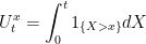
Proof: First note that ${U^x_t}$ is a continuous local martingale starting at zero. Although it is not essential for the proof, it simplifies things a bit to use the Ito isometry,

$\displaystyle {\mathbb E}\left[(U_t^x)^2\right]={\mathbb E}\left[\int_0^t1_{\{X > x\}}d[M]\right]\le{\mathbb E}\left[[M]_\infty\right],$

showing that ${U^x_t}$ is an ${L^2}$ bounded martingale and, by martingale convergence, the limit ${U^x_\infty=\lim_{t\rightarrow\infty} U^x_t}$ exists. We will let E denote the space of continuous functions ${[0,\infty]\rightarrow{\mathbb R}}$ , with the topology of uniform convergence. So, for each x, the paths ${t\mapsto U^x_t}$ can be considered as a random variable taking values in E. Using d for the supremum metric then, for any ${y > x}$ and positive ${\alpha}$ ,

$\displaystyle \begin{aligned} {\mathbb E}\left[d(U^x,U^y)^\alpha\right] &={\mathbb E}\left[\sup_{t\ge0}\left\lvert U^y_t-U^x_t\right\rvert^\alpha\right]\\ &\le C_\alpha{\mathbb E}\left[[U^y-U^x]_t^{\alpha/2}\right]. \end{aligned}$

(3)

This used the BDG inequality, so that ${C_\alpha}$ is a fixed positive constant. Next, we will apply Ito’s formula to the convex function,

$\displaystyle \begin{aligned} &f(X)=(X\wedge y-x)_+^2+2(y-x)(X-y)_+,\\ &f^\prime(X)=2(X\wedge y - x)_+,\\ &f^{\prime\prime}(X)=2 1_{\{y\ge X > x\}}. \end{aligned}$

Although this is not twice continuously differentiable, Ito’s formula still applies by approximating with smooth functions giving,

$\displaystyle \begin{aligned} f(X_t) =&f(X_0)+\int_0^t f^\prime(X_-)dX+\frac12\int_0^t f^{\prime\prime}(X)d[M]\\ &\quad+\sum_{s\le t}(\Delta f(X_s)-f^\prime(X_{s-})\Delta X_s). \end{aligned}$

By convexity of ${f}$ , the final summation is positive. Also, noting that

$\displaystyle \frac12\int_0^t f^{\prime\prime}(X)d[M]=\int_0^t1_{\{y\ge X > x\}}d[M]=[U^y-U^x]_t,$

we obtain the inequality

$\displaystyle [U^y-U^x]_t\le f(X_t)-f(X_0)-\int_0^t f^\prime(X_-)dX.$

Let V be the variation process of A. Using the fact that ${f^\prime(X)}$ is bounded by ${2(y-x)}$ , this gives

$\displaystyle \begin{aligned} {}[U^y-U^x]_t &\le2(y-x)\left(\lvert X_t-X_0\rvert+\left\lvert\int_0^t\xi dM\right\rvert+V_t\right)\\ &\le2(y-x)\left(\lvert M_t-M_0\rvert+\left\lvert\int_0^t\xi dM\right\rvert+2V_t\right) \end{aligned}$

for some process ${\xi}$ bounded by 1. Raising to the power of ${\alpha/2}$ and taking expectations,

$\displaystyle {\mathbb E}\left[[U^y-U^x]_t^{\alpha/2}\right]\le 6^{\alpha/2}(y-x)^{\alpha/2}{\mathbb E}\left[2C_{\alpha/2}[M]_t^{\alpha/4}+2^{\alpha/2}V^{\alpha/2}_t\right]$

Once again, the BDG inequality was used for the expectation of the first two terms in the parantheses on the right hand side. So, ${C_{\alpha/2}}$ is a positive constant. Combining with (3) gives,

$\displaystyle {\mathbb E}\left[d(U^x,U^y)^\alpha\right] \le\tilde C_\alpha(y-x)^{\alpha/2}$

(4)

for the positive constant

$\displaystyle \tilde C_\alpha=C_\alpha6^{\alpha/2}{\mathbb E}\left[2C_{\alpha/2}[M]^{\alpha/4}_\infty+2^{\alpha/2}V_\infty^{\alpha/2}\right].$

Now, Kolmogorov’s continuity theorem can be applied with ${\beta=\alpha/2-1}$ , so long as ${\alpha > 2}$ . This guarantees the existence of a modification of ${U^x}$ which, for all ${\gamma < 1/2-1/\alpha}$ , is locally ${\gamma}$ -Hölder continuous . Finally, note that from the definition, ${U^x_t}$ can be chosen constant in x over the range ${x < \min_tX_t}$ and, similarly, over ${x > \max_t X_t}$ . So, it is constant for x outside of the range ${[\min_tX_t,\max_tX_t]}$ and, hence, is globally ${\gamma}$ -Hölder continuous. Letting ${\alpha}$ increase to infinity, this holds for all ${\gamma < 1/2}$ . ⬜

Localization extends the result above extends to all semimartingales satisfying Hypothesis A.

Lemma 8 Let X be a semimartingale satisfying Hypothesis A, and M be as in decomposition (1). Then, ${U^x_t}$ , defined by (2) has a version which is jointly continuous in t and x. Furthermore, over any bounded range for t, this version is almost surely ${\gamma}$ -Hölder continuous in x for all ${\gamma < 1/2}$ .

Proof: As it satisfies Hypothesis A, we can decompose ${X=M+A}$ for a continuous local martingale M and FV process A. Next, choose a sequence of stopping times, ${\tau_n}$ , increasing to infinity and such that ${[M]^{\tau_n}}$ and the variation of the pre-stopped processes ${A^{\tau_n-}}$ are all bounded. For example, letting V be the variation process of A, we can take

$\displaystyle \tau_n=\inf\left\{t\ge0\colon[M]_t+V_t\ge n\right\}.$

Then, we can decompose

$\displaystyle X^{\tau_n-}=M^{\tau_n}+A^{\tau_n-}.$

These pre-stopped processes satisfy the conditions of lemma 7 and, hence, there exists jointly continuous versions of the processes

$\displaystyle U^{n,x}_t=\int_0^t1_{\{X^{\tau_n-} > x\}}dM^{\tau_n}.$

However, if we define ${U^x_t}$ by (2) then, by optional stopping of stochastic integrals, ${U^x_t=U^{n,x}_t}$ almost surely, whenever ${\tau_n > t}$ . In particular, this means that ${U^{n,x}_t=U^{m,x}_t}$ almost surely, whenever ${\tau_n > t}$ and ${\tau_m > t}$ . By continuity, this holds simultaneously for all x and all ${t < \tau_m\wedge\tau_n}$ , with probability one. Restricting to the event where this holds, we can therefore define the modification

$\displaystyle U^x_t=U^{n,x}_t$

for all n such that ${\tau_n > t}$ . For any positive time T then, almost surely, we can choose n such that ${\tau_n > T}$ , in which case ${U^x_t=U^{n,x}_t}$ is ${\gamma}$ -Hölder continuous in x, over ${t\le T}$ . ⬜

Applying lemma 8 to the definition of the local time for a continuous local martingale immediately provides a jointly continuous modification.

Proof of Theorem 1: By definition, the local times of a continuous semimartingale are given by,

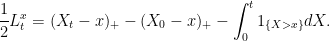$\displaystyle \frac12L^x_t=(X_t-x)_+-(X_0-x)_+-\int_0^t1_{\{X > x\}}dX.$

(5)

As X is a continuous local martingale, we can take ${M=X}$ in lemma 8, so that the integral above as a version which is jointly continuous in t and x, and which is ${\gamma}$ -Hölder continuous in x for all ${\gamma < 1/2}$ and over all bounded intervals for t. We use this version to define the local times ${L^x_t}$ . As all the terms on the right hand side of the above equality satisfy these continuity conditions, the same is true for ${L^x_t}$ . ⬜

In the case of Brownian motion, the proof of lemma 7 can be extended to give joint Hölder continuity.

Lemma 9 Let X be a standard Brownian motion with arbitrary starting value. Then,

$\displaystyle U^x_t=\int_0^t1_{\{X > x\}}dX$

has a version which is jointly continuous in x and t. Furthermore, with probability 1, this is jointly ${\gamma}$ -Hölder continuous over all finite time intervals for t.

Proof: For any ${s < t}$ and ${x\in{\mathbb R}}$ , the BDG inequality gives,

$\displaystyle \begin{aligned} {\mathbb E}\left[\left\lvert U^x_t-U^x_s\right\rvert^\alpha\right] &\le C_\alpha{\mathbb E}\left[\left\lvert[U^x]_t-[U^x]_s\right\rvert^{\alpha/2}\right]\\ &\le C_\alpha{\mathbb E}\left[\left(\int_s^t1_{\{X_u > x\}}du\right)^{\alpha/2}\right]\\ &\le C_\alpha(t-s)^{\alpha/2} \end{aligned}$

for a positive constant ${C_\alpha}$ . For any fixed time ${T\ge0}$ , the stopped process ${X^T}$ satisfies the conditions of lemma 7. So, by (4), there exists a positive constant ${\tilde C}$ such that, for all ${x,y\in{\mathbb R}}$ and ${s,t\in[0,T]}$ ,

$\displaystyle \begin{aligned} {\mathbb E}\left[\lvert U^x_t-U^y_s\rvert^\alpha\right] &\le2^\alpha{\mathbb E}\left[\lvert U^x_t-U^x_s\rvert^\alpha+\lvert U^y_s-U^x_s\rvert^\alpha\right]\\ &\le2^\alpha C_\alpha\lvert t-s\rvert^{\alpha/2}+2^\alpha\tilde C\lvert y-x\rvert^{\alpha/2}. \end{aligned}$

Choosing ${\alpha > 4}$ and ${\beta=\alpha/2-2}$ , the Kolmogorov continuity theorem provides a jointly continuous version of ${U^x_t}$ over ${t\le T}$ , which is locally ${\gamma}$ -Hölder continuous for all ${\gamma < 1/2-2/\alpha}$ . Letting ${\alpha}$ go to infinity, this holds for all ${\gamma < 1/2}$ . Also, as argued in the proof of lemma 7, the fact that ${U^x_t}$ is constant in x for large positive, and large negative, values of x means that it will be globally ${\gamma}$ -Hölder continuous. Finally, the result follows by letting T go to infinity. ⬜

The proof of theorem 2 follows from the lemma above in a very similar way that the proof of theorem 1 followed from lemma 8.

Proof of Theorem 2: We again express the local time using (5). Since we know that the path of a Brownian motion is locally almost surely ${\gamma}$ -Hölder continuous for all ${\gamma < 1/2}$ , it follows that ${(X_t-x)_+}$ is jointly ${\gamma}$ -Hölder continuous in t and x, over bounded time intervals. By lemma 9, the same is true of ${U^x_t}$ and, hence, of ${L^x_t}$ . ⬜

I finally complete the proof of theorem 6, showing that Hypothesis A is sufficient for local times to have a modification that is jointly continuous in time and cadlag in the level. The idea is similar to that given above for continuous local martingales but, now, we have additional terms to account for the jumps of the process and the drift V. In particular, the drift can introduce discontinuities, explaining why we only obtain cadlag versions in x.

Proof of Theorem 6: Let us define ${f_x(X)=(X-x)_+}$ . By definition, the local times are given by

$\displaystyle \frac12L^x_t=f_x(X_t)-f_x(X_s)-\int_0^t1_{\{X_- > x\}}dX-\sum_{s\le t}\left(\Delta f_x(X_s)-1_{\{X_- > x\}}\Delta X_s\right).$

We let M and V be as in decomposition (1).

$\displaystyle \begin{aligned} \frac12L^x_t&=A^x_t-U^x_t-B^x_t,\\ A^x_t&=f_x(X_t)-f_x(X_0)-\sum_{s\le t}\Delta f_x(X_s),\\ U^x_t&=\int_0^t1_{\{X > x\}}dM,\\ B^x_t&=\int_0^t1_{\{X > x\}}dV. \end{aligned}$

Each of the terms on the right hand side can be defined pathwise, except for the stochastic integral ${U^x_t}$ which, by lemma 8, has a jointly continuous version. So, it only remains to check joint continuity for A and B.

Starting with A, for each fixed x, this is a cadlag process with jump ${\Delta f_x(X_t)-\Delta f_x(X_t)}$ , so is continuous. Joint continuity will follow if we can prove uniform continuity in x for t restricted to any bounded interval ${[0,T]}$ . Choosing ${y > x}$ , then the function ${g(X)=f_x(X)-f_y(X)}$ is bounded by ${y-x}$ and has derivative bounded by 1. Hence,

$\displaystyle A^x_t-A^y_t=g(X_t)-g(X_0)-\sum_{s\le t}\Delta g(X_s)$

gives the bound

$\displaystyle \sup_{t\le T}\lvert A^y_t-A^x_t\rvert\le\vert y-x\rvert+\sum_{t\le T}\lvert y-x\rvert\wedge\lvert\Delta X_t\rvert.$

By Hypothesis A, ${\sum_{t\le T}\lvert\Delta X_t\rvert}$ is almost surely bounded and then, by dominated convergence, ${\sup_{t\le T}\lvert A^y_t-A^x_t\rvert}$ tends uniformly to zero as ${y-x\rightarrow0}$ . So ${A^x_t}$ is almost surely uniformly continuous in x over the range ${t\le T}$ , as required.

Finally, we look at ${B^x_t}$ , which we consider to be defined in a pathwise sense. That is, for each fixed ${\omega\in\Omega}$ define it as the pathwise Lebesgue-Stieltjes integral with respect to the locally finite variation path ${t\mapsto V_t(\omega)}$ . For each x, it is an integral with respect to a continuous FV process, so is continuous in t. To complete the proof, we need to show that it is jointly continuous in t and cadlag in x. For this, it is sufficient to show that, over each bounded time interval ${[0,T]}$ , the paths ${t\mapsto B^x_t}$ are cadlag in x under uniform convergence. Fix ${x\in{\mathbb R}}$ and choose ${y > x}$ . Then,

$\displaystyle B^x_t-B^y_t=\int_0^t1_{\{y\ge X > x\}}dV$

and, hence,

$\displaystyle \sup_{t\le T}\lvert B^x_t-B^y_t\rvert\le\int_0^T1_{\{y\ge X > x\}}\lvert dV\rvert.$

The integrand tends to zero as y decreases to x so, by bounded convergence, ${\lvert B^x_t-B^y_t\rvert}$ tends uniformly to zero over ${t\le T}$ . This gives right-continuity in x. To show that the left limits exist, define

$\displaystyle B^{x-}_t=\int_0^t1_{\{X\ge x\}}dV.$

Then, for ${y < x}$ we similarly obtain,

$\displaystyle \sup_{t\le T}\lvert B^{x-}_t-B^y_t\rvert\le\int_0^T1_{\{x > X > y\}}\lvert dV\rvert.$

Again, as y increases to x, bounded convergence shows that ${\lvert B^{x-}_t-B^y_t\rvert}$ tends to zero uniformly over ${t\le T}$ . Hence, ${B^x_t}$ is almost surely jointly continuous in t and cadlag in x, so the same holds for ${L^x_t}$ . Finally, using the expression above for ${B^{x-}_t}$ we obtain that the jump w.r.t. x is,

$\displaystyle \begin{aligned} \frac12(L^x_t-L^{x-}_t) &=B^{x-}_t-B^x_t\\ &=\int_0^t1_{\{X\ge x\}}dV-\int_0^t1_{\{X > x\}}dV\\ &=\int_0^t1_{\{X=x\}}dV \end{aligned}$

as required. ⬜

5 thoughts on “Local Time Continuity”

Dongzhou Huang says:

26 March 21 at 4:33 PM

Hi Professor Lowther,

Thank you a lot for your blogs. I am a Ph.D. student who wants to work on stochastic processes. Your blogs are well-written and detailed. Many questions puzzling me were answered after reading your blogs.

But there is still one place I cannot understand. In the last paragraph of the proof of Lemma 7, you wrote:

note that from the definition, U_t^x can be chosen constant in x over the range xmax_t X_t.

If the process X_t is bounded, I can understand. Suppose sup_t |X_t| < K almost surely, then for x K, U_t^x = 0. But if the process X_t is not bounded, I cannot figure out how to choose U_t^x being constant. The main challenge is that the integral int_0^t 1_{ X >x } dM is not pathwise integral.

By the way, would you mind recommending some references about stochastic integral with respect to semimartingale with a jump? I am trying to learn this part of the knowledge in the next month.

Again, a lot of thanks for your blogs.

Best, Dongzhou

1. George Lowther says:
  
  26 March 21 at 5:19 PM
  
  Hi Dongzhou,
  
  Hopefully Theorem 4 of an earlier post clears up your problems with not being pathwise integrable. However, we do not even need to use that.
  For any K, let T be the stopping time when X first hits K or lower. Then, for levels x, y less than K, the integrands agree on [0,T] so, by stopping, U^x=U^y on [0,T]. In particular, U^x=U^y (almost surely) whenever min_t X_t > K.
  
  1. Dongzhou Huang says:
    
    26 March 21 at 8:16 PM
    
    Hi Professor Lowther,
    
    Thank you for your quick reply. Now I can understand. And thank you for letting me know about Theorem 4. I didn’t know it before.
    
Hugo says:

28 May 22 at 3:57 PM

Hello Dr. Lowther,

Thank you for this very interesting post and your blog. I am a PhD student currently working on stochastic diffusions. Do you think that continuity properties such as those of Theorems 1 and 2 could be proved for the local times of a Brownian motion with drift ?

Best regards,
Hugo

1. George Lowther says:
  
  14 June 22 at 2:51 PM
  
  Not in full generality. E.g., reflecting Brownian motion has discontinuous local time (at level 0), but is a Brownian motion with (singular) drift.
  However, in many cases, Girsanov transforms show that continuity will hold if the drift is of the form $\int\xi\,dt$ , for locally square-integrable $\xi$ .

	Harry on Filtrations and Adapted P…
	Anonymous on Analytic Sets
	Daniel on Analytic Sets
	Sid on Martingale Convergence
	northwiz on Preservation of the Local Mart…
	George Lowther on Martingale Convergence
	Sid on Martingale Convergence
	George Lowther on The Burkholder-Davis-Gundy Ine…
	George Lowther on Preservation of the Local Mart…
	northwiz on Preservation of the Local Mart…

Local Time Continuity

Proof of Continuity

Published by George Lowther

5 thoughts on “Local Time Continuity”

Leave a Reply Cancel reply

Proof of Continuity

Like this:

Related

Published by George Lowther

5 thoughts on “Local Time Continuity”

Leave a Reply Cancel reply