The Ito-Tanaka-Meyer Formula

Ito’s lemma is one of the most important and useful results in the theory of stochastic calculus. This is a stochastic generalization of the chain rule, or change of variables formula, and differs from the classical deterministic formulas by the presence of a quadratic variation term. One drawback which can limit the applicability of Ito’s lemma in some situations, is that it only applies for twice continuously differentiable functions. However, the quadratic variation term can alternatively be expressed using local times, which relaxes the differentiability requirement. This generalization of Ito’s lemma was derived by Tanaka and Meyer, and applies to one dimensional semimartingales.

The local time of a stochastic process X at a fixed level x can be written, very informally, as an integral of a Dirac delta function with respect to the continuous part of the quadratic variation ${[X]^{c}}$ ,

$\displaystyle L^x_t=\int_0^t\delta(X-x)d[X]^c.$

(1)

This was explained in an earlier post. As the Dirac delta is only a distribution, and not a true function, equation (1) is not really a well-defined mathematical expression. However, as we saw, with some manipulation a valid expression can be obtained which defines the local time whenever X is a semimartingale.

Going in a slightly different direction, we can try multiplying (1) by a bounded measurable function ${f(x)}$ and integrating over x. Commuting the order of integration on the right hand side, and applying the defining property of the delta function, that ${\int f(X-x)\delta(x)dx}$ is equal to ${f(X)}$ , gives

$\displaystyle \int_{-\infty}^{\infty} L^x_t f(x)dx=\int_0^tf(X)d[X]^c.$

(2)

By eliminating the delta function, the right hand side has been transformed into a well-defined expression. In fact, it is now the left side of the identity that is a problem, since the local time was only defined up to probability one at each level x. Ignoring this issue for the moment, recall the version of Ito’s lemma for general non-continuous semimartingales,

$\displaystyle \begin{aligned} f(X_t)=& f(X_0)+\int_0^t f^{\prime}(X_-)dX+\frac12A_t\\ &\quad+\sum_{s\le t}\left(\Delta f(X_s)-f^\prime(X_{s-})\Delta X_s\right). \end{aligned}$

(3)

where ${A_t=\int_0^t f^{\prime\prime}(X)d[X]^c}$ . Equation (2) allows us to express this quadratic variation term using local times,

$\displaystyle A_t=\int_{-\infty}^{\infty} L^x_t f^{\prime\prime}(x)dx.$

The benefit of this form is that, even though it still uses the second derivative of ${f}$ , it is only really necessary for this to exist in a weaker, measure theoretic, sense. Suppose that ${f}$ is convex, or a linear combination of convex functions. Then, its right-hand derivative ${f^\prime(x+)}$ exists, and is itself of locally finite variation. Hence, the Stieltjes integral ${\int L^xdf^\prime(x+)}$ exists. The infinitesimal ${df^\prime(x+)}$ is alternatively written ${f^{\prime\prime}(dx)}$ and, in the twice continuously differentiable case, equals ${f^{\prime\prime}(x)dx}$ . Then,

$\displaystyle A_t=\int _{-\infty}^{\infty} L^x_t f^{\prime\prime}(dx).$

(4)

Using this expression in (3) gives the Ito-Tanaka-Meyer formula.

The derivation above is clearly far from being rigorous. For one thing, we started with the informal identity (1), which did not even have a well-defined meaning. For another, the local time ${L^x_t}$ is only defined up to almost sure equivalence. That is, only up to probability one. However, (4) involves the value simultaneously at all real x. The arbitrary choice of ${L^x_t}$ on an uncountable collection of zero probability events, one for each x, could affect the value of the integral. So, we still do not have a well-defined expression. In fact, it is not even clear if ${L^x_t}$ is measurable in x. This is the old problem of choosing good versions of stochastic processes except, now, we are concerned with the path as the level x varies, rather than the time index t.

Before giving a rigorous statement of the Ito-Tanaka-Meyer formula, we first need a jointly measurable version of the local times. As usual, we work with respect to a filtered probability space ${(\Omega,\mathcal F,\{\mathcal F_t\}_{t\ge0},{\mathbb P})}$ .

Lemma 1 Let X be a semimartingale and ${t\ge0}$ . Then, the local times ${L^x_t}$ have a version which is jointly measurable. That is,

$\displaystyle \begin{aligned} & {\mathbb R}^+\times\Omega\times{\mathbb R}\rightarrow{\mathbb R},\\ & (t,\omega,x)\mapsto L^x_t(\omega) \end{aligned}$

is continuous and increasing in t and ${\mathcal B({\mathbb R}^+)\otimes\mathcal F\otimes\mathcal B({\mathbb R})}$ -measurable.

So long as a jointly measurable version of the local times is chosen, the Ito-Tanaka-Meyer formula holds.

Theorem 2 (Ito-Tanaka-Meyer) Let X be a semimartingale, ${f\colon{\mathbb R}\rightarrow{\mathbb R}}$ be convex, and ${L^x_t}$ be a jointly measurable version of the local times. Then,

$\displaystyle \begin{aligned} f(X_t)=& f(X_0)+\int_0^t f^\prime(X_-)dX+\frac12\int_{-\infty}^\infty L^x_t\,f^{\prime\prime}(dx)\\ &\quad+\sum_{s\le t}\left(\Delta f(X_s)-f^\prime(X_{s-})\Delta X_s\right) \end{aligned}$ (5)

almost surely, for each ${t\ge0}$ .

This result clearly extends to any ${f}$ which is a linear combination of convex functions. In the earlier post defining local times, we already showed that the final summation in (5) is almost surely finite and, hence, the integral ${\int L^x_t f^{\prime\prime}(dx)}$ is also finite. In fact, it is equal to the term A in lemma 5 of that post. We can always choose a version of ${L^x_t}$ equal to zero over ${\lvert x\rvert > \sup_{s\le t}\lvert X_s\rvert}$ . It is also usually possible to choose ${L^x_t}$ to be almost surely bounded as x varies, which would explain why the integral is finite, but this is not always possible.

The proofs of lemma 1 and theorem 2 will be given further down. For now, we look at some immediate consequences, starting with the following more rigorous version of identity (2). Note that this was used in the informal derivation of the Ito-Tanaka-Meyer formula above. The more rigorous argument is in the opposite direction, using theorem 2 to prove (2).

Theorem 3 Let X be a semimartingale and ${L^x_t}$ be a jointly measurable version of the local times. Then,

$\displaystyle \int_0^t f(X)\,d[X]^c=\int_{-\infty}^\infty L^x_t f(x) dx$ (6)

almost surely, for all ${t\ge0}$ and measurable ${f\colon{\mathbb R}\rightarrow{\mathbb R}}$ which is either nonnegative or bounded.

Proof: Implicit in equation (6) is the statement that ${L^x_tf(x)}$ is almost surely Lebesgue integrable w.r.t. x, when ${f}$ is bounded. This is equivalent to ${\int L^x_t dx}$ being almost surely finite, which is implied by (5) with ${f(x)=x^2}$ .

First, consider nonnegative continuous ${\theta\colon{\mathbb R}\rightarrow{\mathbb R}}$ . Then, we can define convex and twice continuously differentiable ${f\colon{\mathbb R}\rightarrow{\mathbb R}}$ with ${f^{\prime\prime}=\theta}$ . For example, take ${f(x)=\int_0^x(x-y)\theta(y)dy}$ . Comparing Ito’s formula (3) with (5) immediately gives

$\displaystyle \int_0^t\theta(X)\,d[X]^c=\int_{-\infty}^\infty L^x_t\theta(x)\,dx$

almost surely.

We have shown that (6) holds for all nonnegative and continuous ${f\colon{\mathbb R}\rightarrow{\mathbb R}}$ . Furthermore, if ${f_n\colon{\mathbb R}\rightarrow{\mathbb R}}$ is a sequence of bounded nonnegative measurable functions satisfying (6) and, if ${f_n}$ increases to a limit ${f\colon{\mathbb R}\rightarrow{\mathbb R}}$ then, by monotone convergence, ${f}$ also satisfies (6). So, the result follows from the monotone class theorem. ⬜

Applying theorem 3 for the special case ${f(x)=1}$ expresses the continuous quadratic variation as an integral over the local times.

Corollary 4 Let X be a semimartingale and ${L^x_t}$ be a jointly measurable version of the local times. Then,

$\displaystyle [X]^c_t=\int_{-\infty}^\infty L^x_t\,dx$

almost surely, for each ${t\ge0}$ .

Proof Of The Ito-Tanaka-Meyer Formula

The proof of the Ito-Tanaka-Meyer formula is not really difficult. In fact, for the most part, it is straightforward. However, there are some technical obstacles to be overcome, so I will give a brief outline of the idea before diving into the details.

Recall the definition of local times,

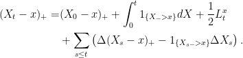$\displaystyle \begin{aligned} (X_t-x)_+= &{}(X_0-x)_++ \int_0^t 1_{\{X_- > x\}}dX +\frac12L^x_t\\ &+\sum_{s\le t}\left(\Delta(X_s-x)_+-1_{\{X_{s-} > x\}}\Delta X_s\right). \end{aligned}$

(7)

The terms in this expression correspond one-to-one with the terms in the target equality (5).

Let ${f(x)}$ be a convex function. For the moment, I assume that it has a bounded derivative and that ${f(x)\rightarrow0}$ as x tends to minus infinity, which simplifies things a bit, and will generalize to arbitrary convex functions afterwards. Then, integrate both sides of (7) w.r.t. ${f^{\prime\prime}(dx)}$ . We will show that each of the terms of (7) has a jointly measurable version, which is integrable over x, and the integral is equal to the corresponding term of (5), which will imply that (7) holds for the given choice of ${f}$ .

The left hand side and the first term on the right are jointly measurable and the integral is easily evaluated,

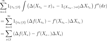
$\displaystyle \begin{aligned} &\int_{-\infty}^\infty (X_t-x)_+ f^{\prime\prime}(dx)= f(X_t),\\ &\int_{-\infty}^\infty (X_0-x)_+ f^{\prime\prime}(dx)= f(X_0). \end{aligned}$

The stochastic Fubini theorem can be applied to the second term on the right. This states that it has a jointly measurable version, which is cadlag in t and integrable over x, and we can commute the order of integration,

$\displaystyle \begin{aligned} \int_{-\infty}^\infty \int_0^t 1_{\{X_- > x\}}dX f^{\prime\prime}(dx) &= \int_0^t \int_{-\infty}^\infty 1_{\{X_- > x\}} f^{\prime\prime}(dx)dX\\ &=\int_0^t f^\prime(X_-)dX. \end{aligned}$

This equals the second term on the right of (5).

The third term on the right hand side of (7) is just the local time. It will automatically have a version which is cadlag in t, jointly measurable, and integrable over x, so long as each of the other terms do, by linearity. Then, the third term on the right of (5) is explicitly equal to the integral of this over x, so we have nothing to prove here.

Now, look at the final term of (7), which accounts for the jumps of X. As it stands, the sum is over the uncountable set of times ${s\le t}$ . To fix this issue, choose a countable sequence, ${\tau_n}$ , of stopping times with disjoint graphs, whose union almost surely contain the jump times of X with probability one. That this is always possible was shown was shown earlier in my notes. Then, the term can be rewritten as

$\displaystyle \sum_{n=1}^\infty1_{\{\tau_n\le t\}}\left(\Delta(X_{\tau_n}-x)_+-1_{\{X_{\tau_n-} > x\}}\Delta X_{\tau_n}\right)$

for all x, almost surely. The summand here is nonnegative, so we can integrate with respect to ${f^{\prime\prime}(dx)}$ and apply the standard Fubini theorem to obtain,

$\displaystyle \begin{aligned} &\sum_{n=1}^\infty1_{\{\tau_n\le t\}}\int\left(\Delta(X_{\tau_n}-x)_+-1_{\{X_{\tau_n-} > x\}}\Delta X_{\tau_n}\right)f^{\prime\prime}(dx)\\ &=\sum_{n=1}^\infty1_{\{\tau_n\le t\}}\left(\Delta f(X_{\tau_n})-f^\prime(X_{\tau_n-})\Delta X_{\tau_n}\right)\\ &=\sum_{s\le t}\left(\Delta f(X_s)-f^\prime(X_{s-})\Delta X_s\right) \end{aligned}$

almost surely. This completes the proof of theorem 2 for the current choice of ${f}$ .

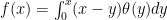
Note that if the function is linear, of the form ${f(x)=ax+b}$ for constants a and b, then (5) is straightforward. As ${f^{\prime\prime}=0}$ it reduces to

$\displaystyle aX_t+b=aX_0+b+\int_0^t a dX,$

which is immediate.

Now consider the case where ${f^{\prime\prime}(x)=0}$ for ${\lvert x\rvert > K}$ , for some constant K. As it is linear over ${x < -K}$ , we can write

$\displaystyle f(x)=\tilde f(x)+ax+b$

for constants a and b, and convex function ${\tilde f(x)}$ which is equal to zero over ${x < -K}$ . By the argument above, (5) holds with ${f(x)}$ replaced by either ${\tilde f(x)}$ or ${ax+b}$ and, by linearity, it holds for ${f}$ .

Finally, consider arbitrary convex ${f}$ . Fixing positive real ${K\ge0}$ , define the function

$\displaystyle \tilde f(x)=\begin{cases} f(x),&{\rm for\ }\lvert x\rvert\le K,\\ f(K)+f^\prime(K+)(x-K),&{\rm for\ }x > K,\\ f(-K)+f^\prime(K-)(x-K),&{\rm for\ }x < -K, \end{cases}$

which is convex and satisfies ${\tilde f(x)=f(x)}$ for ${\lvert x\rvert\le K}$ and ${\tilde f^{\prime\prime}(x)=0}$ otherwise. So, by the argument above, (5) holds for ${f}$ replaced by ${\tilde f}$ . Also, on the event that ${\sup_{s\le t}\lvert X_s\rvert < K}$ , each of the terms of (2) is unchanged under replacing ${f}$ by ${\tilde f}$ . Hence, (5) holds on this event. Letting K increase to infinity completes the proof of theorem 2.

The argument above not only proved the Ito-Tanaka-Meyer formula, it also established the existence of local times which are jointly measurable as stated in lemma 1, and cadlag in t. To complete the proof of lemma 1, it only remains to show that the local times can simultaneously be chosen to be continuous and increasing in t. Consider the set,

$\displaystyle A=\left\{(\omega,x)\in\Omega\times{\mathbb R}\colon t\mapsto L^x_t(\omega){\rm\ is\ continuous\ and\ increasing}\right\}.$

For general processes, this need not be measurable. In our case, we already know that ${t\mapsto L^x_t(\omega)}$ is cadlag, implying that to be continuous and increasing in t is equivalent to it being locally uniformly continuous and increasing for t restricted to the rational numbers. As the rationals are countable, this gives an ${\mathcal F\otimes\mathcal E}$ -measurable set. So,

$\displaystyle \tilde L^x_t(\omega)=1_{\{(\omega,x)\in A\}}L^x_t(\omega)$

gives a jointly measurable version of the local times which is also continuous and increasing in t.

	Harry on Filtrations and Adapted P…
	Anonymous on Analytic Sets
	Daniel on Analytic Sets
	Sid on Martingale Convergence
	northwiz on Preservation of the Local Mart…
	George Lowther on Martingale Convergence
	Sid on Martingale Convergence
	George Lowther on The Burkholder-Davis-Gundy Ine…
	George Lowther on Preservation of the Local Mart…
	northwiz on Preservation of the Local Mart…

The Ito-Tanaka-Meyer Formula

Proof Of The Ito-Tanaka-Meyer Formula

Published by George Lowther

Leave a Reply Cancel reply

Proof Of The Ito-Tanaka-Meyer Formula

Like this:

Related

Published by George Lowther

Leave a Reply Cancel reply