Stochastic Processes, Indistinguishability and Modifications

George Lowther Filtrations and Processes, Stochastic Calculus Notes 3 November 0915 September 20

I start these notes on stochastic calculus with the definition of a continuous time stochastic process. Very simply, a stochastic process is a collection of random variables ${\{X_t\}_{t\ge 0}}$ defined on a probability space ${(\Omega,\mathcal{F},{\mathbb P})}$ . That is, for each time ${t\ge 0}$ , ${\omega\mapsto X_t(\omega)}$ is a measurable function from ${\Omega}$ to the real numbers.

Stochastic processes may also take values in any measurable space ${(E,\mathcal{E})}$ but, in these notes, I concentrate on real valued processes. I am also restricting to the case where the time index ${t}$ runs through the non-negative real numbers ${{\mathbb R}_+}$ , although everything can easily be generalized to other subsets of the reals.

A stochastic process ${X\equiv\{X_t\}_{t\ge 0}}$ can be viewed in either of the following three ways.

As a collection of random variables, one for each time ${t\ge 0}$ .
As a path
$\displaystyle \setlength\arraycolsep{2pt} \begin{array}{rl} &\displaystyle {\mathbb R}_+\rightarrow{\mathbb R},\smallskip\\ &\displaystyle t\mapsto X_t(\omega), \end{array}$

one for each ${\omega\in\Omega}$ . These are referred to as the sample paths of the process.
As a function from the product space
$\displaystyle \setlength\arraycolsep{2pt} \begin{array}{rl} &\displaystyle {\mathbb R}_+\times\Omega\rightarrow{\mathbb R},\smallskip\\ &\displaystyle (t,\omega)\mapsto X_t(\omega). \end{array}$

As is often the case in probability theory, we are not interested in events which occur with zero probability. Stochastic process theory is no different, and two processes ${X,Y}$ are said to be indistinguishable if there is an event ${A\subseteq\Omega}$ of probability one such that ${X_t(\omega)=Y_t(\omega)}$ for all ${\omega\in A}$ and all ${t\ge 0}$ . This is the same as saying that they almost surely (i.e., with probability one) have the same sample paths. Alternative language which is often used is that ${X}$ and ${Y}$ are equivalent up to evanescence. In general, when discussing any properties of a stochastic process, it is common to only care about what holds up to evanescence. For example, if a processes has continuous sample paths with probability one, then it is referred to as a continuous process and we don’t care if it actually has discontinuous paths on some event of zero probability.

It is important to realize that even if we have two processes ${X,Y}$ satisfying ${X_t=Y_t}$ almost surely, at each time ${t}$ , then it does not follow that they are indistinguishable. As an example, consider a random variable ${T}$ uniformly distributed over the interval ${[0,1]}$ , and define the process ${X_t=1_{\{t=T\}}}$ . For each time ${t}$ , ${{\mathbb P}(X_t\not=0)={\mathbb P}(T=t)=0}$ . However, ${X}$ is not indistinguishable from the zero process, as the sample path ${t\mapsto X_t(\omega)}$ always has one point at which ${X}$ takes the value ${1}$ . The problem here is the uncountability of nonnegative real numbers used for the time index. By countable additivity of measures, if ${X_t=Y_t}$ almost surely, for each ${t}$ , then we can infer that the sample paths of ${X}$ and ${Y}$ are almost surely identical on any given countable set of times ${S\subset{\mathbb R}_+}$ , but cannot extend this to uncountable sets.

This necessitates a further definition. A process ${Y}$ is a version or modification of ${X}$ if, for each time ${t\ge 0}$ , ${{\mathbb P}(X_t=Y_t)=1}$ . Alternative language sometimes used is that ${X}$ and ${Y}$ are stochastically equivalent.

Whenever a stochastic process is defined in terms of its values at each individual time ${t}$ , or in terms of its joint distributions at finite times, then replacing it by any other version will still satisfy the definition. It is therefore important to choose a good version. Right-continuous (or left-continuous) versions are often used when possible, as this then defines the process up to evanescence.

Lemma 1 Let ${X}$ and ${Y}$ be right-continuous processes (resp. left-continuous processes) such that ${X_t=Y_t}$ almost surely, at each time ${t\ge 0}$ . Then, they are indistinguishable.

Proof: By countable additivity, the set ${A=\{\omega\colon X_t(\omega)=Y_t(\omega){\rm\ for\ all\ }t\in{\mathbb Q}_+\}}$ has probability one. By right-continuity (resp. left-continuity) of the sample paths, it follows that ${X}$ and ${Y}$ have the same paths for all ${\omega\in A}$ . ⬜

As an example, the definition of a standard Brownian motion ${W}$ consists of two parts. First, ${W_0=0}$ and, for ${t>s}$ , ${W_t-W_s}$ is normal with mean 0 and variance ${t-s}$ , independently of ${\{W_u\}_{0\le u\le s}}$ , which defines its finite distributions. The additional condition that it has continuous sample paths is required in order to select the correct version up to evanescence.

Viewing a stochastic process in the third sense mentioned above, as a function on the product space ${{\mathbb R}_+\times\Omega}$ , it is often necessary to impose a measurability condition. The process ${X}$ is said to be jointly measurable if it is measurable with respect to the product sigma-algebra ${\mathcal{B}({\mathbb R}_+)\otimes\mathcal{F}}$ . Here, ${\mathcal{B}}$ denotes the Borel sigma-algebra. Another benefit of choosing left or right-continuous versions is that it ensures joint measurability.

Lemma 2 All right-continuous and left-continuous processes are jointly measurable.

Proof: If ${X}$ is right-continuous, then it is the limit of the following sequence of processes

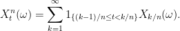
$\displaystyle X^n_t(\omega) = \sum_{k=1}^\infty 1_{\{(k-1)/n\le t< k/n\}}X_{k/n}(\omega).$

Clearly ${(t,\omega)\mapsto 1_{\{(k-1)/n\le t <k/n\}}X_{k/n}(\omega)}$ are jointly measurable functions and, therefore, ${X=\lim_{n\rightarrow\infty}X^n}$ is also jointly measurable.

The proof for left-continuous processes follows along the same lines, but using ${X_{(k-1)/n}}$ in place of ${X_{k/n}}$ . ⬜

Finally, it is often useful to sample a stochastic process at a random time. The value of a process ${X}$ at the measurable time ${\tau\colon\Omega\rightarrow{\mathbb R}_+}$ is ${X_{\tau(\omega)}(\omega)}$ . This need not even be a measurable quantity unless a good version of the process is used. Fortunately, joint measurability of ${X}$ is enough.

Lemma 3 If ${X}$ is jointly measurable and ${\tau\colon\Omega\rightarrow{\mathbb R}_+}$ is a random time then ${X_\tau}$ is measurable.

Proof: Using the functional monotone class theorem, it is only necessary to prove the result for processes ${X_t(\omega)=1_{\{(t,\omega)\in B\times F\}}}$ with ${B\in\mathcal{B}({\mathbb R}_+)}$ and ${F\in\mathcal{F}}$ . However, ${X_{\tau(\omega)}(\omega)=1_{\{\omega\in\tau^{-1}(B)\cap F\}}}$ is clearly measurable. ⬜

Published by George Lowther

View all posts by George Lowther

Published 3 November 0915 September 20

30 thoughts on “Stochastic Processes, Indistinguishability and Modifications”

songqsh says:

27 April 10 at 1:21 AM

Dear Almost sure,
It is in fact a nicely written note.
In Lemma 2 above, I am wondering if you need to add an additional assumption.
For instance, Let $Y$ is non-measurable random variable w.r.t $(\Omega, \mathcal{F}, \mathbb{F})$ .
Setting process $X_t(\omega) = Y(\omega)$ , then $X$ is not jointly measurable function, although it is continuous.
Best
songqsh

Reply
1. George Lowther says:
  
  27 April 10 at 3:58 AM
  
  Thanks for your comment. If X is a stochastic process, then it is implicit that X_t is a random variable (i.e., it is measurable) for each time t. This rules out your example.
  I’ll come back and try to clarify the statement when I have some time.
  
  Reply
  1. songqsh says:
    
    27 April 10 at 6:30 AM
    
    Thank you for quick response. It clarifies my question.
    
    Reply
TheBridge says:

16 June 10 at 10:31 AM

Dear Almost Sure,

I have recently discovered your blog and wanted to congratulate you warmly for this work.

Regarding Lemma 3, as you have proven Joint Measurability is sufficient condition for $X_\tau$ to be well defined random variable.

Is there any reason why you didn’t mention progressive measurability, which is, as far as I know, the sharpest condition for this random variable to make sense.

Best Regards and “encore bravo”

Reply
1. George Lowther says:
  
  17 June 10 at 12:56 PM
  
  TheBridge – Welcome
  
  Actually, progressive measurability implies joint measurability. So, joint measurability is a weaker condition, giving a stronger result.
  
  Besides, progressive measurability only makes sense when you have a filtration and is only really needed when $\tau$ is a stopping time. In that case, you get the stronger conclusions that the stopped process $X^\tau$ is progressive (hence jointly measurable and adapted) and that $X_\tau$ is $\mathcal{F}_\tau$ -measurable.
  
  See also my later posts about this (Filtrations and adapted processes, Stopping times and the debut theorem and Sigma algebras at a stopping time).
  
  Regards,
  George
  
  Reply
Alex says:

13 March 11 at 2:08 AM

Dear Dr.Lowther,
thank you for these notes. However, I have a question. What should we require from a function f so that the process f(X_t) is progressively measurable if X_t is progressively measurable? Is it a well-known result?
Thank you in advance.
Sincerely,
Alex.

Reply
1. George Lowther says:
  
  13 March 11 at 2:49 AM
  
  As compositions of measurable functions are measurable, you just need f to be Borel measurable.
  
  Reply
Alex says:

27 August 11 at 5:37 AM

Dear Dr.Lowther,
as usual I use your notes to undertstand concepts that are not well-written in books. I’m trying to write a complete proof of Lemma 3 and I have a question. If we look at the Functional Monotone Class Theorem on PlanetMath then using the same notation K – the space of simple functions, but what is H then?
Thank you.
Sincerely,
Alex.

Reply
1. George Lowther says:
  
  27 August 11 at 1:28 PM
  
  Hi. Try taking H to be the space of all processes X such that $X_\tau$ is measurable. Then, H contains the simple functions and is closed under taking linear combinations and taking pointwise limits of sequences. The monotone class theorem implies that H contains all jointly measurable processes. Strictly speaking, directly applying the monotone class theorem tells you that H contains all bounded and jointly measurable processes, but extending to unbounded ones is not difficult (by taking limits of bounded processes or looking at $H/(1+\vert H\vert)$ ).
  
  Reply
Des Yeev says:

22 November 11 at 9:44 PM

Dear Almost Sure

I found this nice site accidentally. I really appreciate.
In your simple proof of Lemma 1, you used a countable set for t. Is here a good place to say something about continuity issues like separable process?
Thanks a lot.
Yeev

Reply
1. George Lowther says:
  
  22 November 11 at 11:39 PM
  
  Hi.
  I was really only looking at processes with nice modifications here, such has right-continuous processes. As you need to have measurable quantities, and we deal with countably additive measures, it is natural to try and look at quantities which are defined over a finite set of times. Using right-continuity allows you to express quantities in terms of the restriction to a countable index set. This also seems to be the idea behind the notion of separable processes (Springer Online Reference), although it is not really something that I have really looked at before. Certainly, the right-continuous processes are separable relative to the closed subsets of R. Is there much of a gain in formalizing the more general concept?
  
  George
  
  Reply
Marcelo Fernandes says:

31 May 12 at 6:24 AM

I still learning about stochastic theory, this are being helpful a lot to me.

Reply
1. George Lowther says:
  
  6 June 12 at 2:24 AM
  
  Glad these notes are helpful, and thanks for the comment!
  
  Reply
Marco says:

11 July 12 at 8:56 PM

Hi, this is probably obvious but just occurred to me recently, while looking at a problem concerning indistinguishability but given two any two processes how do we know that the set
{X_t=Y_t, for all t>=0} is measurable? It is obviously the intersection of the measurable sets {X_t=Y_t} for all t>= but this is of course an uncountable intersection. Would appreciate any feedback. By the way your blog is excellent and handier than Revuz and Yor. Also are you are interested in non-linear expectations, BSDEs and risk measures and thinking of adding some notes of these topics to your blog?

Reply
1. George Lowther says:
  
  13 July 12 at 12:05 AM
  
  The set {X_t = Y_t} need not be measurable. However, the property of processes being indistinguishable still makes sense. You can take measurability of the set (w.r.t. the completion of the probability space) as being part of the definition. So, if the set is not measurable, then the processes are not indistinguishable. Also, as long as both X and Y are jointly measurable then the set will be measurable.
  
  I haven’t really thought much about the topics you mention for this blog. However, I’m not sure what I might add in the future, so maybe, at some point.
  
  Reply
Amos Lapidoth says:

20 July 12 at 9:47 AM

Dear Almost Sure,
I am looking for conditions that guarantee the existence of a Stochastic Process of given FDDs that is measurable with respect to the product of the sigma-algebra generated by its cylindrical sets and the Borel algebra on the real line. Continuity in probability suffices for the existence of a measurable SP but not necessarily with the respect to this product of sigma-algebras.
I am particularly interested in the Normal case. Given an autcovariance function that is continuous at the origin, does there always exists a centered stationary Normal stochastic process of this autocovariance function that is measurable with respect to the product of the cylindrical sigma-algebra and the Borel algebra on the real line? If not, are you away of any sufficient conditions that guarantee this?

Reply
1. George Lowther says:
  
  6 September 12 at 2:02 AM
  
  Hi,
  
  Sorry, I don’t have any references for this. I would guess that some kind of uniform continuity in probability should be enough (but I don’t have a reference for that statement). Consider choosing a sequence ε_n of positive reals tending to zero fast enough that X(t_n) → X(t) almost surely, for any sequence of times with |t_n – t| ≤ ε. Then approximate X by the piecewise constant process Xⁿ(t) = X(ε_n[t/ε_n]). Then takes limits as n goes to infinity to get a jointly measurable modification of X.
  
  Reply
Marcelo de Almeida says:

23 August 13 at 5:39 AM

Reblogged this on Being simple.

Reply
Dimas Abreu Dutra says:

5 February 14 at 8:13 PM

Dear George, does it also makes sense to say that two real-valued random variables are indistinguishable if they are almost surely equal?

Reply
Quasar says:

3 November 14 at 11:23 AM

Hi George – I am new to Stochastic Calculus. I have basic knowledge of probability and statistics. However, I find it difficult to understand term like probability space, measure etc. Are there any pre-requisites?

Reply
Pingback: Cauchy-Schwarz inequality for bilinear forms valued in an abstract vector space - MathHub
Anonymous says:

2 December 16 at 4:57 AM

Hi George, I have two questions and need your help. First in Lemma 1, X and Y are right-continuous process, and for each t, X almost surely equals Y, but t is uncountable, so why the set A has the probability 1 and what’s the function of right-continuous version here? Second, in Lemma 2, I don’t understand the meaning of ‘measurable w.r.t. product sigma-algebra’, can you explain it for me? looking forward to your reply, and thank you very much!

Reply
1. George Lowther says:
  
  9 December 16 at 2:40 AM
  
  1) The point of restricting the statement to right-continuous (or left-continuous) processes is that, for X to equal Y everywhere, it is only necessary to show that this holds on the rationals. Taking right-limits extends the equality to irrational t. And, the rationals are countable, so the processes will be equal on the rationals, almost surely.
  2) We have two sigma algebras. The Borel sigma algebra on the positive reals $\mathcal{B}(\mathbb{R}_+)$ , and the sigma algebra $\mathcal{F}$ on the underlying probability space. A (real) stochastic process is a map $\mathbb{R}_+\times\Omega\to\mathbb{R}$ . measurable w.r.t. the product sigma algebra means measurable with respect to $\mathcal{B}(\mathbb{R}_+)\otimes\mathcal{F}$ in the domain and $\mathcal{B}(\mathbb{R})$ in the codomain.
  
  Reply
ADRIAN HINOJOSA CALLEJA says:

5 April 17 at 11:21 AM

Really nice note, as usual this webpage is very useful, thank you very much and congratulations!

Reply
David A Kozak says:

19 May 17 at 6:44 PM

Hello sir,

First, this blog is much appreciated. I couldn’t believe my luck finding such a comprehensive and easy-to-understand compendium on a topic that seems to be pretty scarcely populated with resources. I’m working my way through to your treatment of Quasi-martingales because the only other resource I’ve found on discrete-time quasi-martingales is by Metivier, and his book is inaccessible.

Second, I have a (perhaps naive) question. How is $\tau$ in lemma (3) a function of $\Omega$ ? I can see $X_\tau$ taking an input $\omega$ and returning a value in $\mathbb{R}$ , but $\tau$ itself shouldn’t necessarily take any inputs unless I’m missing something entirely?

Thank you again,
David

Reply
1. David A Kozak says:
  
  19 May 17 at 6:45 PM
  
  Also, apologies, I’ve no idea how to get the TeX markup to work…
  
  Reply
2. David A Kozak says:
  
  19 May 17 at 7:57 PM
  
  Aha as I consider how stopping times work, specifically the description in the Stopping Times section, I retract my question. Further apologies for the spam.
  
  Reply
  1. George Lowther says:
    
    20 May 17 at 1:12 PM
    
    No problem. Also I fixed your latex (https://almostsure.wordpress.com/using-latex-in-comments/)
    
    Reply
Sam says:

27 July 18 at 7:22 AM

Dear George,

Great post, I find your blog touch on a wide range of topics most conventional textbooks don’t cover. In fact that’s how I came about this website looking for results working on left right limit processes (more specifically optional semimartingales). I’m wondering if you can point me towards any textbooks or papers which discusses/proves the results in this post on stochastic processes with left right limits and also textbooks that discusses in depth predictive, optional, progressive measurable and adapted processes. Thanks in advance!

Sam

Reply
Wei Miao says:

10 July 20 at 8:45 PM

Dear George,

Thanks for the detailed notes here! I wonder whether there is any work on distinguishing two stochastic processes in the collection of r.v.’s sense. What technique and what condition should we have in order to uniquely determine a stochastic process that is continuous in the r.v. sense?

Reply

	Anonymous on About
	Anonymous on About
	Anonymous on The Stochastic Integral
	Anonymous on Bessel Processes
	Anonymous on Bessel Processes
	Stat Prof on Pathwise Regularity of Optiona…
	Yang Chu on Spitzer’s Formula
	Anonymous on About
	Anonymous on Continuous Processes with Inde…
	Anonymous on Continuous Processes with Inde…

Related

Published by George Lowther

30 thoughts on “Stochastic Processes, Indistinguishability and Modifications”

Leave a comment Cancel reply