
Fubini’s theorem states that, subject to precise conditions, it is possible to switch the order of integration when computing double integrals. In the theory of stochastic calculus, we also encounter double integrals and would like to be able to commute their order. However, since these can involve stochastic integration rather than the usual deterministic case, the classical results are not always applicable. To help with such cases, we could do with a new stochastic version of Fubini’s theorem. Here, I will consider the situation where one integral is of the standard kind with respect to a finite measure, and the other is stochastic. To start, recall the classical Fubini theorem.
Theorem 1 (Fubini) Let
and
be finite measure spaces, and
be a bounded
-measurable function. Then,
is
-measurable,
is
-measurable, and,
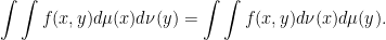
(1)

I previously gave a proof of this as a simple corollary of the functional monotone class theorem. Note that the first two statements regarding measurability of the single integrals are necessary to ensure that the double integral (1) is well-defined. There are various straightforward ways in which this base statement can be generalized. By simple linearity, it extends to finite signed measure spaces. Alternatively, by monotone convergence, we can extend to sigma-finite measure spaces and nonnegative measurable functions 
A slight reformulation of Fubini’s theorem is useful for applications to stochastic calculus. Here, we work with respect to a probability space 
Theorem 2 Let X be an FV process,
be a uniformly bounded collection of processes such that
is
-measurable. Then,
(2) is
measurable,
(3) is
(4) for each
.


Proof: For each individual value of 

![{[0,t]}](https://s0.wp.com/latex.php?latex=%7B%5B0%2Ct%5D%7D&bg=ffffff&fg=000000&s=0&c=20201002)

First, define 
 |
This is
Measurability of (3) is a bit more tricky, and the dependence of X on 


 |
This is 

The result stated in theorem 2 only applies to FV processes, whereas stochastic integration is defined more generally for semimartingales. Generalizing to semimartingales does introduce some technical problems though. First, it is necessary that the integrand is predictable. That is, it should be measurable with respect to the predictable sigma-algebra 
Lemma 3 Let
is
-measurable. Then, the process
is bounded and predictable.
Proof: It is clear that 

 |
is
The next technical difficulty in giving a stochastic version of Fubini’s theorem is that if
 |
is only defined up to probability one. Therefore, asking if it is measurable with respect to x does not even make sense. Furthermore, the arbitrary choice of the value of the integral on an uncountable collection of zero probability events, one for each x, could affect the value of the integral over x. This is the old problem of choosing good versions of stochastic processes except, now, we are concerned with the path as the variable x varies, rather than the time index t.
Lemma 4 Let
be a measurable space and
such that
(5) almost surely, for each t and x, and such that
is

This result depends on choosing a good version of the stochastic integral, simultaneously for all values of x, which is a bit tricky, so is left until later. We can now give a precise statement of the generalization of Fubini’s theorem for stochastic integration with respect to a semimartingale.
Theorem 5 (Stochastic Fubini Theorem) Let X be a semimartingale,
be a real-valued, bounded, and
be as given by lemma 4. Then,
is almost surely finite and,
(6) almost surely.

In the statement, the fact that 
Before moving on to the proof of this theorem, there is a small ambiguity to be cleared up. We know that certain pathwise properties of stochastic processes, such as continuity, are sufficient to prove that the version is unique up to evanescence. Joint measurability is not sufficient by itself, so there will generally be many non-equivalent versions of the stochastic integral satisfying the conclusion of lemma 4. In fact, it does not matter which version is chosen in (6), as they will all give the same result when we perform the integral.
Lemma 6 Let
be collections of nonnegative random variables which are jointly measurable, in the sense that
are
-measurable. If
almost surely, for each
then, with probability one,
almost all x.
To be precise, there exists
of probability one and, for each
, there exists a set
of full
for all
.
In particular, if the random variables are nonnegative then,
almost surely.


Proof: As the integral does not depend on the values of the integrand on a null set, the ‘in particular’ part of the theorem follows immediately from the first statement. We just need to show that, with probability one,
![\displaystyle {\mathbb E}\left[\int\lvert U^x-V^x\rvert d\mu(x)\right]= \int{\mathbb E}\left[\lvert U^x-V^x\rvert\right]d\mu(x) =0.](https://s0.wp.com/latex.php?latex=%5Cdisplaystyle++%7B%5Cmathbb+E%7D%5Cleft%5B%5Cint%5Clvert+U%5Ex-V%5Ex%5Crvert+d%5Cmu%28x%29%5Cright%5D%3D+%5Cint%7B%5Cmathbb+E%7D%5Cleft%5B%5Clvert+U%5Ex-V%5Ex%5Crvert%5Cright%5Dd%5Cmu%28x%29+%3D0.+&bg=ffffff&fg=000000&s=0&c=20201002) |
As any nonnegative random variable is almost surely zero, if its expected value is zero, we see that
 |
almost surely. In this case, 
Existence of Measurable Integrals
I we give a proof of lemma 4, showing that we can always choose a jointly measurable version of the stochastic integral. The proof is along similar lines to Protter, Stochastic Integration and Differential Equations. We start with the following result showing that certain limits of jointly measurable processes themselves have jointly measurable versions.
Lemma 7 Let
be random variables for
such that
is
(uniform convergence on compacts in probability) as n goes to infinity, for each x.
Then,
has a version which is

Proof: In order to measure the rate of convergence, consider the pseudometric defining the ucp topology,
![\displaystyle D(X-Y)=\sum_{k=1}^\infty{\mathbb E}\left[2^{-k}\wedge\sup_{s\le k}\lvert X_s-Y_s\rvert\right].](https://s0.wp.com/latex.php?latex=%5Cdisplaystyle++D%28X-Y%29%3D%5Csum_%7Bk%3D1%7D%5E%5Cinfty%7B%5Cmathbb+E%7D%5Cleft%5B2%5E%7B-k%7D%5Cwedge%5Csup_%7Bs%5Cle+k%7D%5Clvert+X_s-Y_s%5Crvert%5Cright%5D.+&bg=ffffff&fg=000000&s=0&c=20201002) |
Then, define
 |
which, by ucp convergence, decreases to zero as n goes to infinity. Using ucp convergence again,
 |
which, by joint measurability of 
Now, for any fixed 


 |
From the definition, this is jointly measurable and cadlag in t. For any 
 |
Hence, for each positive integer m, replacing 


 |
for all
 |
As this is the expectation of
 |
this sum has finite expectation and, so, is almost surely finite for each x. Let 

 |
By construction, this is cadlag in t and is 


Lemma 7 can be applied to complete the proof of lemma 4.
Proof of Lemma 4: We will use the functional monotone class theorem, so define 


 |
Choosing a cadlag version of the stochastic integral, this is
By the monotone class theorem, it just remains to show that, if 
By the assumption that
 |
to be 
Proof of the Stochastic Fubini Theorem
I now give a proof of theorem 5. One method used, for example by Protter in Stochastic Integration and Differential Equations, is to decompose the semimartingale into FV and local martingale terms. It can then be proved separately for these two cases, and combined to give the full result. However, in keeping with much of my stochastic calculus notes, I take a different approach. This will avoid relying on any semimartingale decompositions, and keep closer to our original definition of stochastic integration. However, whichever way we go about it, handling the various limits does get a bit tricky. The main tool used here will be Ito’s formula. For a semimartingale X and twice continuously differentiable 
![\displaystyle \begin{aligned} f(X_t)&=f(X_0)+\int_0^t f^\prime(X_-)dX+\frac12\int_0^t f^{\prime\prime}(X_-)d[X]^{c}\\ &+\sum_{s\le t}(\Delta f(X_s)-f^\prime(X_{s-})\Delta X_s). \end{aligned}](https://s0.wp.com/latex.php?latex=%5Cdisplaystyle++%5Cbegin%7Baligned%7D+f%28X_t%29%26%3Df%28X_0%29%2B%5Cint_0%5Et+f%5E%5Cprime%28X_-%29dX%2B%5Cfrac12%5Cint_0%5Et+f%5E%7B%5Cprime%5Cprime%7D%28X_-%29d%5BX%5D%5E%7Bc%7D%5C%5C+%26%2B%5Csum_%7Bs%5Cle+t%7D%28%5CDelta+f%28X_s%29-f%5E%5Cprime%28X_%7Bs-%7D%29%5CDelta+X_s%29.+%5Cend%7Baligned%7D+&bg=ffffff&fg=000000&s=0&c=20201002) |
In addition, we will suppose that 


![\displaystyle \left\lvert f(X_t)-f(X_0)-\int_0^tf^\prime(X_-)dX\right\rvert\le L[X]_t.](https://s0.wp.com/latex.php?latex=%5Cdisplaystyle++%5Cleft%5Clvert+f%28X_t%29-f%28X_0%29-%5Cint_0%5Etf%5E%5Cprime%28X_-%29dX%5Cright%5Crvert%5Cle+L%5BX%5D_t.+&bg=ffffff&fg=000000&s=0&c=20201002) |
Consequently, if we furthermore suppose that 


![\displaystyle \left\lvert f(U_t)-\int_0^t\xi f^\prime(U_-)dX\right\rvert\le L\int_0^t\xi^2 d[X]\le L[X]_t](https://s0.wp.com/latex.php?latex=%5Cdisplaystyle++%5Cleft%5Clvert+f%28U_t%29-%5Cint_0%5Et%5Cxi+f%5E%5Cprime%28U_-%29dX%5Cright%5Crvert%5Cle+L%5Cint_0%5Et%5Cxi%5E2+d%5BX%5D%5Cle+L%5BX%5D_t+&bg=ffffff&fg=000000&s=0&c=20201002) |
(7) |
almost surely. The main part of the proof of theorem 5 consists of extending this inequality to incorporate an integral over the auxiliary parameter x.
Lemma 8 Let X be a semimartingale,
If
(8) almost surely, for each
![\displaystyle \left\lvert\int f(U^x_t)d\mu(x)-\int_0^t\int\xi^xf^\prime(U^x_-)d\mu(x)dX\right\rvert\le L[X]_t](https://s0.wp.com/latex.php?latex=%5Cdisplaystyle++%5Cleft%5Clvert%5Cint+f%28U%5Ex_t%29d%5Cmu%28x%29-%5Cint_0%5Et%5Cint%5Cxi%5Exf%5E%5Cprime%28U%5Ex_-%29d%5Cmu%28x%29dX%5Cright%5Crvert%5Cle+L%5BX%5D_t+&bg=ffffff&fg=000000&s=0&c=20201002)
Proof: Note that all of the integrands in (8) are bounded and, hence, integrable. To prove the bound, we use the functional monotone class theorem. So, let
 |
for a finite sequence of pairwise disjoint sets 


 |
which is jointly measurable as required. Then,
 |
We obtain,
![\displaystyle \begin{aligned} &\left\lvert\int f(U^x_t)d\mu(x)-\int_0^t\int\xi^xf^\prime(U^x_-)d\mu(x)dX\right\rvert\\ &= \left\lvert\sum_{k=1}^n\mu(A_k)\left(f(V^k_t)-\int_0^t\zeta^kf^\prime(V^k_-)dX\right)\right\rvert\\ &\le \sum_{k=1}^n\mu(A_k)L[X]_t\le L[X]_t. \end{aligned}](https://s0.wp.com/latex.php?latex=%5Cdisplaystyle++%5Cbegin%7Baligned%7D+%26%5Cleft%5Clvert%5Cint+f%28U%5Ex_t%29d%5Cmu%28x%29-%5Cint_0%5Et%5Cint%5Cxi%5Exf%5E%5Cprime%28U%5Ex_-%29d%5Cmu%28x%29dX%5Cright%5Crvert%5C%5C+%26%3D+%5Cleft%5Clvert%5Csum_%7Bk%3D1%7D%5En%5Cmu%28A_k%29%5Cleft%28f%28V%5Ek_t%29-%5Cint_0%5Et%5Czeta%5Ekf%5E%5Cprime%28V%5Ek_-%29dX%5Cright%29%5Cright%5Crvert%5C%5C+%26%5Cle+%5Csum_%7Bk%3D1%7D%5En%5Cmu%28A_k%29L%5BX%5D_t%5Cle+L%5BX%5D_t.+%5Cend%7Baligned%7D+&bg=ffffff&fg=000000&s=0&c=20201002) |
The first inequality here used (7), and the second used the fact that 

Next, suppose that 

![\displaystyle \begin{aligned} &{\mathbb E}\left[\int1\wedge\sup_{s\le t}\lvert U^{x,n}_s-U^x_s\rvert d\mu(x)\right]\\ &=\int{\mathbb E}\left[1\wedge\sup_{s\le t}\lvert U^{x,n}_s-U^x_s\rvert\right] d\mu(x) \rightarrow0 \end{aligned}](https://s0.wp.com/latex.php?latex=%5Cdisplaystyle++%5Cbegin%7Baligned%7D+%26%7B%5Cmathbb+E%7D%5Cleft%5B%5Cint1%5Cwedge%5Csup_%7Bs%5Cle+t%7D%5Clvert+U%5E%7Bx%2Cn%7D_s-U%5Ex_s%5Crvert+d%5Cmu%28x%29%5Cright%5D%5C%5C+%26%3D%5Cint%7B%5Cmathbb+E%7D%5Cleft%5B1%5Cwedge%5Csup_%7Bs%5Cle+t%7D%5Clvert+U%5E%7Bx%2Cn%7D_s-U%5Ex_s%5Crvert%5Cright%5D+d%5Cmu%28x%29+%5Crightarrow0+%5Cend%7Baligned%7D+&bg=ffffff&fg=000000&s=0&c=20201002) |
as n goes to infinity. So, by passing to a subsequence if necessary, we can assume that
![\displaystyle {\mathbb E}\left[\int1\wedge\sup_{s\le t}\lvert U^{x,n}_s-U^x_s\rvert d\mu(x)\right]\le2^{-n}.](https://s0.wp.com/latex.php?latex=%5Cdisplaystyle++%7B%5Cmathbb+E%7D%5Cleft%5B%5Cint1%5Cwedge%5Csup_%7Bs%5Cle+t%7D%5Clvert+U%5E%7Bx%2Cn%7D_s-U%5Ex_s%5Crvert+d%5Cmu%28x%29%5Cright%5D%5Cle2%5E%7B-n%7D.+&bg=ffffff&fg=000000&s=0&c=20201002) |
In particular, this means that
 |
has finite expectation, so is almost surely finite. Furthermore, when this is finite then 

 |
hold for all
![\displaystyle \begin{aligned} &\left\lvert\int f(U^x_t)d\mu(x)-\int_0^t\int\xi^xf^\prime(U^x_-)d\mu(x)dX\right\rvert\\ &=\lim_{n\rightarrow\infty}\left\lvert\int f(U^{x,n}_t)d\mu(x)-\int_0^t\int\xi^{x,n}f^\prime(U^{x,n}_-)d\mu(x)dX\right\rvert\\ &\le L[X]_t \end{aligned}](https://s0.wp.com/latex.php?latex=%5Cdisplaystyle++%5Cbegin%7Baligned%7D+%26%5Cleft%5Clvert%5Cint+f%28U%5Ex_t%29d%5Cmu%28x%29-%5Cint_0%5Et%5Cint%5Cxi%5Exf%5E%5Cprime%28U%5Ex_-%29d%5Cmu%28x%29dX%5Cright%5Crvert%5C%5C+%26%3D%5Clim_%7Bn%5Crightarrow%5Cinfty%7D%5Cleft%5Clvert%5Cint+f%28U%5E%7Bx%2Cn%7D_t%29d%5Cmu%28x%29-%5Cint_0%5Et%5Cint%5Cxi%5E%7Bx%2Cn%7Df%5E%5Cprime%28U%5E%7Bx%2Cn%7D_-%29d%5Cmu%28x%29dX%5Cright%5Crvert%5C%5C+%26%5Cle+L%5BX%5D_t+%5Cend%7Baligned%7D+&bg=ffffff&fg=000000&s=0&c=20201002) |
almost surely. So,
This shows that, if we let 

I finally apply lemma 8 to complete the proof of theorem 5.
Proof of Theorem 5: By scaling, without loss of generality, we assume that 


![\displaystyle \limsup_{n\rightarrow\infty}\left\lvert\int f_n(U^{x,n}_t)d\mu(x)-\int_0^t\int\xi^xf^\prime_n(U^{x}_-)d\mu(x)dX\right\rvert\le L[X]_t,](https://s0.wp.com/latex.php?latex=%5Cdisplaystyle++%5Climsup_%7Bn%5Crightarrow%5Cinfty%7D%5Cleft%5Clvert%5Cint+f_n%28U%5E%7Bx%2Cn%7D_t%29d%5Cmu%28x%29-%5Cint_0%5Et%5Cint%5Cxi%5Exf%5E%5Cprime_n%28U%5E%7Bx%7D_-%29d%5Cmu%28x%29dX%5Cright%5Crvert%5Cle+L%5BX%5D_t%2C+&bg=ffffff&fg=000000&s=0&c=20201002) |
(9) |
almost surely. Furthermore, by bounded convergence, the second integral on the left hand side of (9) converges in probability to 
In particular, if 


Finally, consider 

 |
almost surely, as required. ⬜

Hi, in the last formula of Lemma 6, , the integral bounds
  and
and  does not make sense, since the integral is over arbitrary measure space
  . Are they typos or am I missing something?
No, you are not missing anything. I fixed it now, thanks!