In stochastic calculus it is common to work with processes adapted to a filtered probability space  . As with probability space extensions, It can sometimes be necessary to enlarge the underlying space to introduce additional events and processes. For example, many diffusions and local martingales can be expressed as an integral with respect to Brownian motion but, sometimes, it may be necessary to enlarge the space to make sure that it includes a Brownian motion to work with. Also, in the theory of stochastic differential equations, finding solutions can sometimes require enlarging the space.
Extending a probability space is a relatively straightforward concept, which I covered in an earlier post. Extending a filtered probability space is the same, except that it also involves enlarging the filtration  . It is important to do this in a way which does not destroy properties of existing processes, such as their distributions conditional on the filtration at each time.
Let’s consider a filtered probability space  . An enlargement
is, firstly, an extension of the probability spaces. It is a map from Ω′ to Ω measurable with respect to  and
and  , and preserving probabilities. So ℙ′(π-1E) = π(E) for all
  . In addition, it is required to be
  measurable for each time t ≥ 0, meaning that
  for all
  . Consequently, any adapted process Xt lifts to an adapted process X∗t = π∗Xt on the larger space, defined by X∗t(ω) = Xt(π(ω)).
As with extensions of probability spaces, this can be considered in two steps. First, we extend to the filtered probability space on Ω′ with induced sigma-algebra  consisting of sets π-1E for , and to the filtration
  . This is essentially a no-op, since events and random variables on the original filtered probability space are in one-to-one correspondence with those on the enlarged space, up to zero probability events. Next, the sigma-algebras are enlarged to
  and
and  . This is where new random events are added to the event space and filtration.
Such arbitrary extensions are too general for many uses in stochastic calculus where we merely want to add in some additional source of randomness. Consider, for example, a standard Brownian motion B defined on the original space so that, for any times s < t, Bt – Bs is normal and independent of  . Does it necessarily lift to a Brownian motion on the enlarged space? The answer to this is no! It need not be the case that B∗t – B∗s is independent of
  . For an extreme case, consider the situation where
  and π is the identity, so there is no enlargement of the sample space. If the filtration is is extended to the maximum,
  , consider what happens to our Brownian motion. The increment Bt – Bs is -measurable, so is not independent of it. In fact, conditioned on
  , the entire path of B is deterministic. It is definitely not a Brownian motion with respect to this new filtration. Similarly, martingales, submartingales and supermartingales will not remain as such if we pass to this enlarged filtration.
The idea is that, if ![{ Y={\mathbb E}[X\vert\mathcal F_t]}](https://s0.wp.com/latex.php?latex=%7B+Y%3D%7B%5Cmathbb+E%7D%5BX%5Cvert%5Cmathcal+F_t%5D%7D&bg=ffffff&fg=000000&s=0&c=20201002) for random variables X, Y defined on our original probability space, then this relation should continue to hold in the extension. It is required that
for random variables X, Y defined on our original probability space, then this relation should continue to hold in the extension. It is required that ![{ Y^*={\mathbb E}[X^*\vert\mathcal F'_t]}](https://s0.wp.com/latex.php?latex=%7B+Y%5E%2A%3D%7B%5Cmathbb+E%7D%5BX%5E%2A%5Cvert%5Cmathcal+F%27_t%5D%7D&bg=ffffff&fg=000000&s=0&c=20201002) . This is exactly relative independence of
. This is exactly relative independence of  and over .
Recall that two sigma-algebras  and
and  are relatively independent over a third
  if
if
for all  and
and  . The following properties are each equivalent to this definition;
![{{\mathbb E}[XY\vert\mathcal K]={\mathbb E}[X\vert\mathcal K]{\mathbb E}[Y\vert\mathcal K]}](https://s0.wp.com/latex.php?latex=%7B%7B%5Cmathbb+E%7D%5BXY%5Cvert%5Cmathcal+K%5D%3D%7B%5Cmathbb+E%7D%5BX%5Cvert%5Cmathcal+K%5D%7B%5Cmathbb+E%7D%5BY%5Cvert%5Cmathcal+K%5D%7D&bg=ffffff&fg=000000&s=0&c=20201002) for all bounded -measurable random variables X and -measurable Y.
for all bounded -measurable random variables X and -measurable Y.![{{\mathbb E}[X\vert\mathcal G]={\mathbb E}[X\vert\mathcal K]}](https://s0.wp.com/latex.php?latex=%7B%7B%5Cmathbb+E%7D%5BX%5Cvert%5Cmathcal+G%5D%3D%7B%5Cmathbb+E%7D%5BX%5Cvert%5Cmathcal+K%5D%7D&bg=ffffff&fg=000000&s=0&c=20201002) for all bounded -measurable X.
for all bounded -measurable X.![{{\mathbb E}[X\vert\mathcal H]={\mathbb E}[X\vert\mathcal K]}](https://s0.wp.com/latex.php?latex=%7B%7B%5Cmathbb+E%7D%5BX%5Cvert%5Cmathcal+H%5D%3D%7B%5Cmathbb+E%7D%5BX%5Cvert%5Cmathcal+K%5D%7D&bg=ffffff&fg=000000&s=0&c=20201002) for all bounded -measurable X.
for all bounded -measurable X.
This leads us to the idea of a standard extension of filtered probability spaces.
Definition 1 An extension of filtered probability spaces
is standard if, for each time t ≥ 0, the sigma-algebras and are relatively independent over .
Continue reading “Extending Filtered Probability Spaces” →


![\displaystyle {\mathbb P}(A\cap B) = {\mathbb E}\left[{\mathbb P}(A\vert\mathcal K){\mathbb P}(B\vert\mathcal K)\right]](https://s0.wp.com/latex.php?latex=%5Cdisplaystyle+%7B%5Cmathbb+P%7D%28A%5Ccap+B%29+%3D+%7B%5Cmathbb+E%7D%5Cleft%5B%7B%5Cmathbb+P%7D%28A%5Cvert%5Cmathcal+K%29%7B%5Cmathbb+P%7D%28B%5Cvert%5Cmathcal+K%29%5Cright%5D+&bg=ffffff&fg=000000&s=0&c=20201002)


 . This is the common issue of choosing good
 -Hölder continuous w.r.t. x, for all
  and over all bounded regions for t.
 ![{[X]^{c}}](https://s0.wp.com/latex.php?latex=%7B%5BX%5D%5E%7Bc%7D%7D&bg=ffffff&fg=000000&s=0&c=20201002) ,
,![\displaystyle L^x_t=\int_0^t\delta(X-x)d[X]^c.](https://s0.wp.com/latex.php?latex=%5Cdisplaystyle++L%5Ex_t%3D%5Cint_0%5Et%5Cdelta%28X-x%29d%5BX%5D%5Ec.+&bg=ffffff&fg=000000&s=0&c=20201002)
 and integrating over x. Commuting the order of integration on the right hand side, and applying the defining property of the delta function, that
  is equal to
  , gives
![\displaystyle \int_{-\infty}^{\infty} L^x_t f(x)dx=\int_0^tf(X)d[X]^c.](https://s0.wp.com/latex.php?latex=%5Cdisplaystyle++%5Cint_%7B-%5Cinfty%7D%5E%7B%5Cinfty%7D+L%5Ex_t+f%28x%29dx%3D%5Cint_0%5Etf%28X%29d%5BX%5D%5Ec.+&bg=ffffff&fg=000000&s=0&c=20201002)
![{A_t=\int_0^t f^{\prime\prime}(X)d[X]^c}](https://s0.wp.com/latex.php?latex=%7BA_t%3D%5Cint_0%5Et+f%5E%7B%5Cprime%5Cprime%7D%28X%29d%5BX%5D%5Ec%7D&bg=ffffff&fg=000000&s=0&c=20201002) . Equation (
. Equation (
 , it is only really necessary for this to exist in a weaker, measure theoretic, sense. Suppose that
  exists, and is itself of locally finite variation. Hence, the Stieltjes integral
  exists. The infinitesimal
  is alternatively written
  and, in the twice continuously differentiable case, equals
  . Then,
 and
and  be finite measure spaces, and
  be a bounded
  -measurable function. Then,
 -measurable, and,
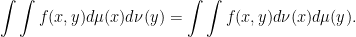
 to denote the running maximum of a process.
![{{\mathbb P}\left(\bar X_t \ge K\right)\le K^{-1}{\mathbb E}[X_t]}](https://s0.wp.com/latex.php?latex=%7B%7B%5Cmathbb+P%7D%5Cleft%28%5Cbar+X_t+%5Cge+K%5Cright%29%5Cle+K%5E%7B-1%7D%7B%5Cmathbb+E%7D%5BX_t%5D%7D&bg=ffffff&fg=000000&s=0&c=20201002) for all
for all  .
. for all
  .
.![{{\mathbb E}[\bar X_t]\le(e/(e-1)){\mathbb E}[X_t\log X_t+1]}](https://s0.wp.com/latex.php?latex=%7B%7B%5Cmathbb+E%7D%5B%5Cbar+X_t%5D%5Cle%28e%2F%28e-1%29%29%7B%5Cmathbb+E%7D%5BX_t%5Clog+X_t%2B1%5D%7D&bg=ffffff&fg=000000&s=0&c=20201002) .
.
![\displaystyle {\mathbb P}(\bar X_t\ge K)\le\inf_{x < K}\frac{{\mathbb E}[(X_t-x)_+]}{K-x}.](https://s0.wp.com/latex.php?latex=%5Cdisplaystyle++%7B%5Cmathbb+P%7D%28%5Cbar+X_t%5Cge+K%29%5Cle%5Cinf_%7Bx+%3C+K%7D%5Cfrac%7B%7B%5Cmathbb+E%7D%5B%28X_t-x%29_%2B%5D%7D%7BK-x%7D.+&bg=ffffff&fg=000000&s=0&c=20201002)
 , there exists a martingale with this terminal distribution for which (
 in (
in (![\displaystyle {\mathbb E}[F(\bar X_t)]\le{\mathbb E}[G(X_t)]](https://s0.wp.com/latex.php?latex=%5Cdisplaystyle++%7B%5Cmathbb+E%7D%5BF%28%5Cbar+X_t%29%5D%5Cle%7B%5Cmathbb+E%7D%5BG%28X_t%29%5D+&bg=ffffff&fg=000000&s=0&c=20201002)
 . The aim of this post is to show how they have a more general `pathwise’ form,
 . It is relatively straightforward to show that (
 will be of the form
  for an increasing right-continuous function
  , so
, so 
 , so can be used as the definition of
  . In the case where X is a semimartingale, integration by parts ensures that this agrees with the stochastic integral
  . Since we now have an interpretation of (
 to be a cadlag real-valued function. Hence, we reduce the martingale inequalities to straightforward results of real-analysis not requiring any probability theory and, consequently, are much more general. I state the precise pathwise generalizations of Doob’s inequalities now, leaving the proof until later in the post. As the first of inequality of theorem
  ,
,
 .
. then,
then,
 .
.
 .
.
 is a measure of the time spent at x. For a continuous time stochastic process, we could try and simply compute the Lebesgue measure of the time at the level,
 and stick there for some time, this makes some sense. However, if X is a standard
  at each positive time, so that that
  defined by (
 as in (
![{{\mathbb E}[\delta(X_s-x)]}](https://s0.wp.com/latex.php?latex=%7B%7B%5Cmathbb+E%7D%5B%5Cdelta%28X_s-x%29%5D%7D&bg=ffffff&fg=000000&s=0&c=20201002) can be interpreted as the probability density of
can be interpreted as the probability density of  evaluated at
 ![\displaystyle L^x_t=\int_0^t\delta(X_s-x)d[X]_s](https://s0.wp.com/latex.php?latex=%5Cdisplaystyle++L%5Ex_t%3D%5Cint_0%5Et%5Cdelta%28X_s-x%29d%5BX%5D_s+&bg=ffffff&fg=000000&s=0&c=20201002)

![{\int f^{\prime\prime}(X)d[X]}](https://s0.wp.com/latex.php?latex=%7B%5Cint+f%5E%7B%5Cprime%5Cprime%7D%28X%29d%5BX%5D%7D&bg=ffffff&fg=000000&s=0&c=20201002) and, hence, requires
and, hence, requires  can be understood in terms of distributions, and delta functions can appear, which brings local times into the picture. In the opposite direction, which I take in this post, we can try to generalise Ito’s formula and invert this to give a meaning to (
 such that
  is convex in x and right-continuous and decreasing in t, is
  necessarily a semimartingale? It was explained how this is equivalent to the
 ![{f\colon[0,1]^2\rightarrow{\mathbb R}}](https://s0.wp.com/latex.php?latex=%7Bf%5Ccolon%5B0%2C1%5D%5E2%5Crightarrow%7B%5Cmathbb+R%7D%7D&bg=ffffff&fg=000000&s=0&c=20201002) such that
such that  where
where  and
and  are convex in x and increasing in t. This is the form of the hypothesis which this post will be concerned with, so the example will only involve simple real analysis and no stochastic calculus. I will give some numerical calculations suggesting that the construction below is a counterexample, but do not have any proof of this. So, the hypothesis is still open.
![{\{M_t\}_{t\in[0,1]}}](https://s0.wp.com/latex.php?latex=%7B%5C%7BM_t%5C%7D_%7Bt%5Cin%5B0%2C1%5D%7D%7D&bg=ffffff&fg=000000&s=0&c=20201002) is the martingale constructed there, then
is the martingale constructed there, then![\displaystyle C(t,x)={\mathbb E}[(M_t-x)_+]](https://s0.wp.com/latex.php?latex=%5Cdisplaystyle++C%28t%2Cx%29%3D%7B%5Cmathbb+E%7D%5B%28M_t-x%29_%2B%5D+&bg=ffffff&fg=000000&s=0&c=20201002)
![{[0,1]\times[-1,1]}](https://s0.wp.com/latex.php?latex=%7B%5B0%2C1%5D%5Ctimes%5B-1%2C1%5D%7D&bg=ffffff&fg=000000&s=0&c=20201002) to
to  which is convex in x and increasing in t. The question is then whether C can be expressed as the difference of functions which are convex in x and decreasing in t. The example constructed in this post will be the same as C with the time direction reversed, and with a linear function of x added so that it is zero at
  .
. 
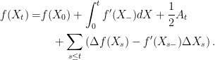
 . In the case where f is twice continuously differentiable then the process V is given by
 ![\displaystyle \setlength\arraycolsep{2pt} \begin{array}{rl} \displaystyle [X]_t&\displaystyle=[X]^c_t+\sum_{s\le t}(\Delta X_s)^2,\smallskip\\ \displaystyle [X,Y]_t&\displaystyle=[X,Y]^c_t+\sum_{s\le t}\Delta X_s\Delta Y_s. \end{array}](https://s0.wp.com/latex.php?latex=%5Cdisplaystyle++%5Csetlength%5Carraycolsep%7B2pt%7D+%5Cbegin%7Barray%7D%7Brl%7D+%5Cdisplaystyle+%5BX%5D_t%26%5Cdisplaystyle%3D%5BX%5D%5Ec_t%2B%5Csum_%7Bs%5Cle+t%7D%28%5CDelta+X_s%29%5E2%2C%5Csmallskip%5C%5C+%5Cdisplaystyle+%5BX%2CY%5D_t%26%5Cdisplaystyle%3D%5BX%2CY%5D%5Ec_t%2B%5Csum_%7Bs%5Cle+t%7D%5CDelta+X_s%5CDelta+Y_s.+%5Cend%7Barray%7D+&bg=ffffff&fg=000000&s=0&c=20201002)
![{[X]^c}](https://s0.wp.com/latex.php?latex=%7B%5BX%5D%5Ec%7D&bg=ffffff&fg=000000&s=0&c=20201002) , is zero. As the only difference between the
, is zero. As the only difference between the ![{[X]^c=0}](https://s0.wp.com/latex.php?latex=%7B%5BX%5D%5Ec%3D0%7D&bg=ffffff&fg=000000&s=0&c=20201002) .
. ![{[X,Y]^c=0}](https://s0.wp.com/latex.php?latex=%7B%5BX%2CY%5D%5Ec%3D0%7D&bg=ffffff&fg=000000&s=0&c=20201002) for all semimartingales Y.
for all semimartingales Y. ![{[X,Y]=0}](https://s0.wp.com/latex.php?latex=%7B%5BX%2CY%5D%3D0%7D&bg=ffffff&fg=000000&s=0&c=20201002) for all continuous semimartingales Y.
for all continuous semimartingales Y. ![{[X,M]=0}](https://s0.wp.com/latex.php?latex=%7B%5BX%2CM%5D%3D0%7D&bg=ffffff&fg=000000&s=0&c=20201002) for all continuous local martingales M.
for all continuous local martingales M.  for a
for a  of FV processes such that
  in the
 ![{\bar{\mathbb R}_+=[0,\infty]}](https://s0.wp.com/latex.php?latex=%7B%5Cbar%7B%5Cmathbb+R%7D_%2B%3D%5B0%2C%5Cinfty%5D%7D&bg=ffffff&fg=000000&s=0&c=20201002) . Stopping a process can only decrease its mean variation (recall the alternative definitions
. Stopping a process can only decrease its mean variation (recall the alternative definitions 

 , so in this case the following result says that stopped martingales are martingales.
 be a simple stopping time. Then


